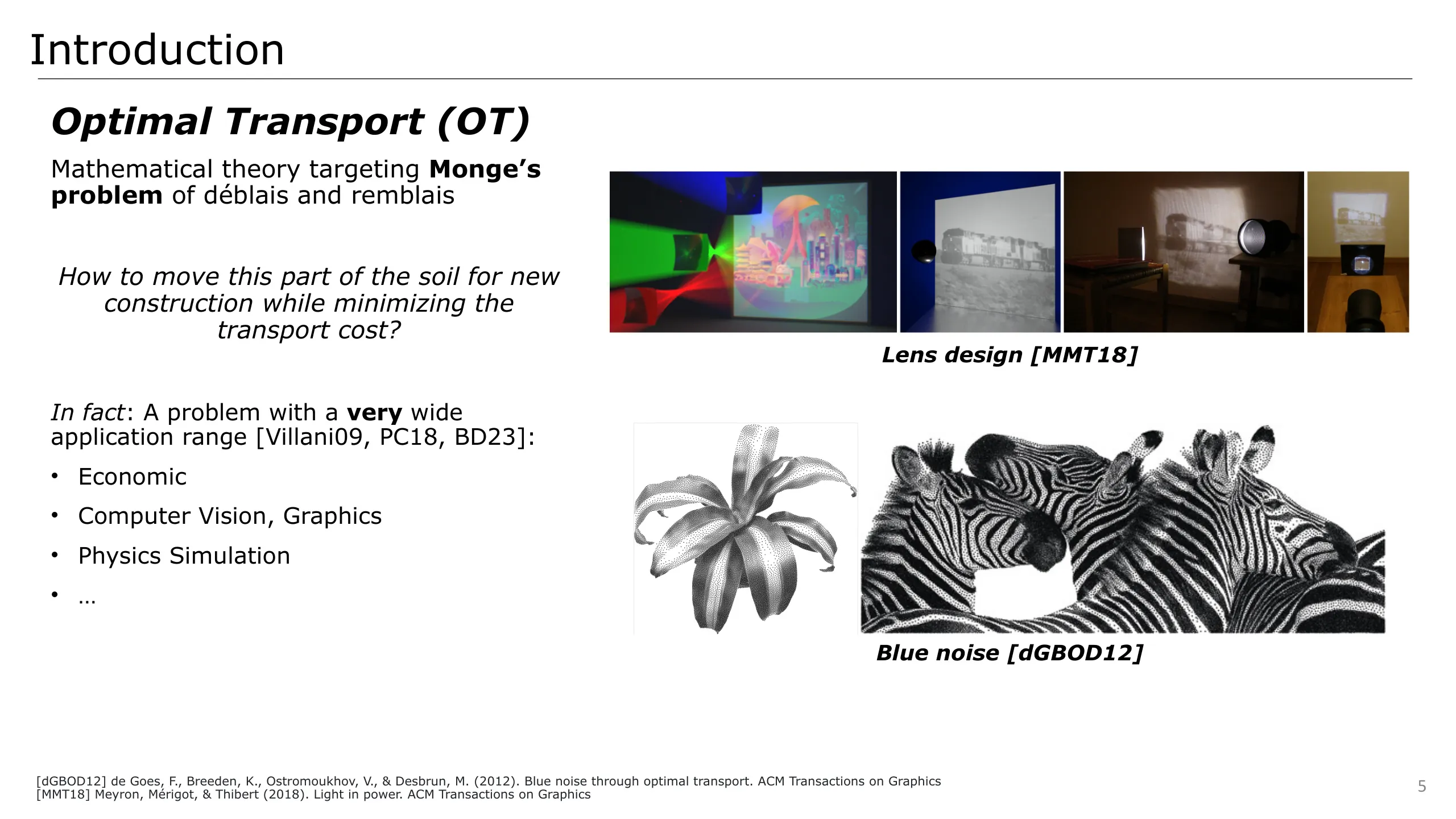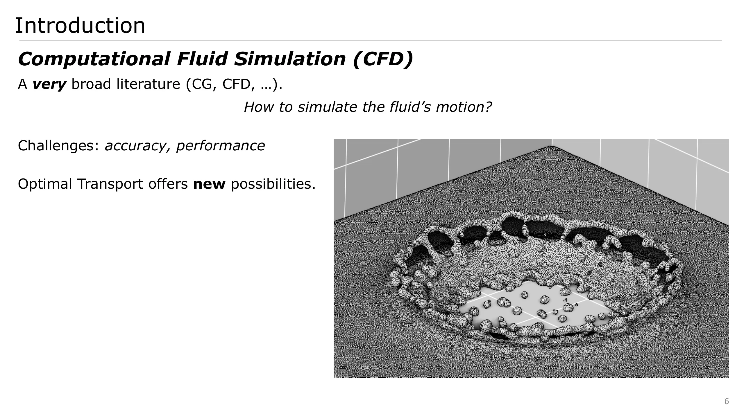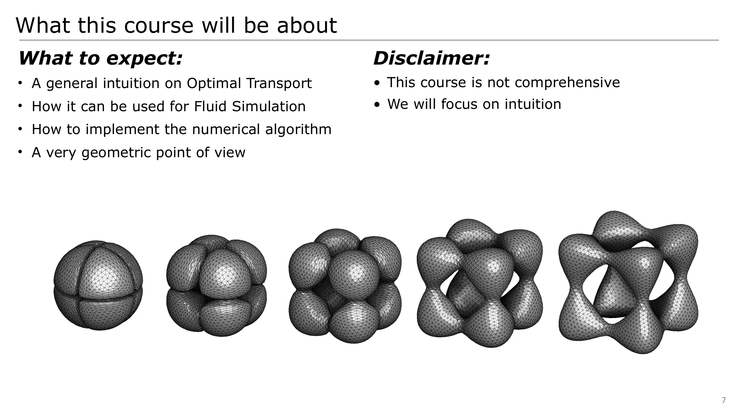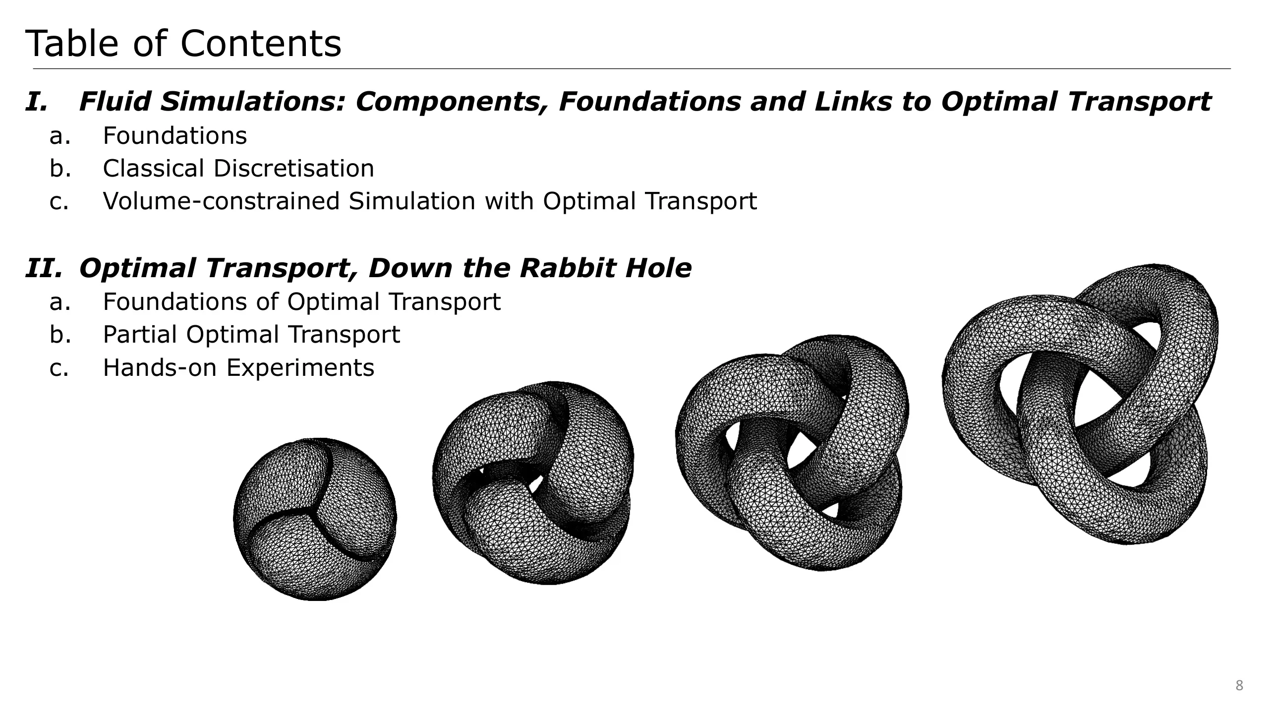
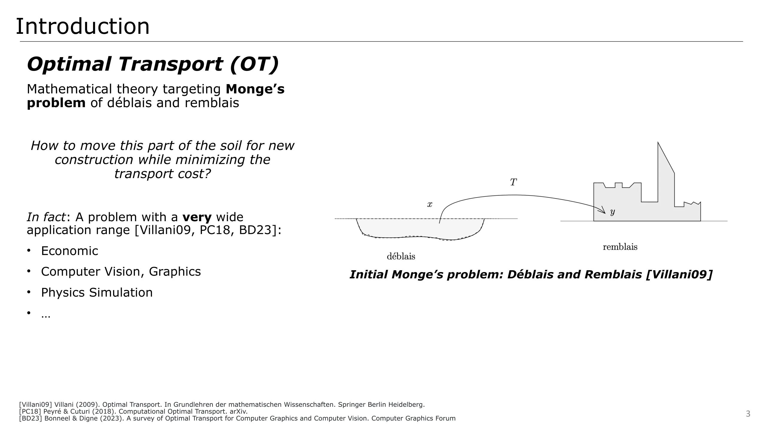
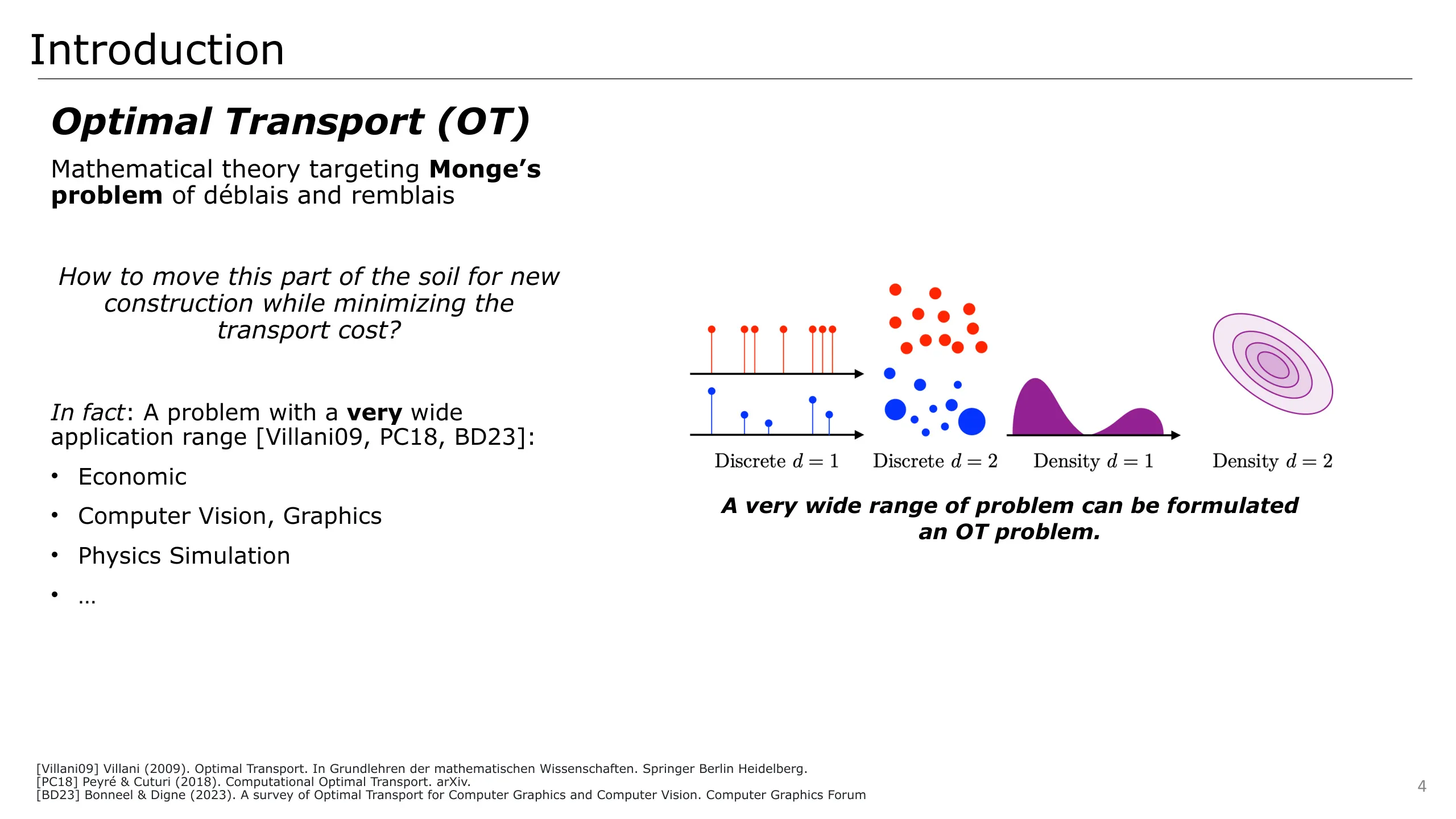
Optimal Transport for Fluid Simulation: New and Old

Optimal Transport is a very general mathematical theory

The origin story is Gaspard Monge, working for the army, who wanted to reduce the cost of moving the soil from one place to another for construction

This problem has been proved as applicable in a very wide application range: economic, computer vision or graphics, numerical simulation…

- This important problem has been studied by a lot of people. Here, I give a few examples of interesting works in graphics for lens design or blue noise.

In this course, we will discuss the use of Optimal Transport for fluid simulation.

This is also a wide subject, targeting the numerical simulation of the motion of the fluid matter, realistically.

Here, we want accuracy and performance. In such context OT provides a new framework for such simulation as we will see

We also wish to clarify first the goals of this course.

We want to provide:

- A general intuition on Optimal Transport, s.t. it makes sense when to use it and how to implement a solver targeting a specific case

- What are its links with fluid simulation and how to implement it

- All of that with a very geometric point of view to develop intuition

We also want to highlight that:

- As both subjects are quite wide, the presentation will not be comprehensive

- We will rather focus on providing an intuition

So the course will be split in two main parts:

- The first one will focus on the background on fluid simulations

- This will start with some theoretical foundations, to understand what will be our tools

- Which will be followed by the discretisation we will have to perform to actually compute the simulation on a computer and the classical ways to do it

- Finally, we will show how those are linked to Optimal Transport

- The second one will focus on the actual optimal transport problem

- And then how a partial optimal transport problem actually fits to the problem of free surface simulation

- Finally, we will do some hands-on experiments

So first of all, let’s define the mathematical tools we will use to describe the matter

To actually simulate the motion of the matter we will have to:

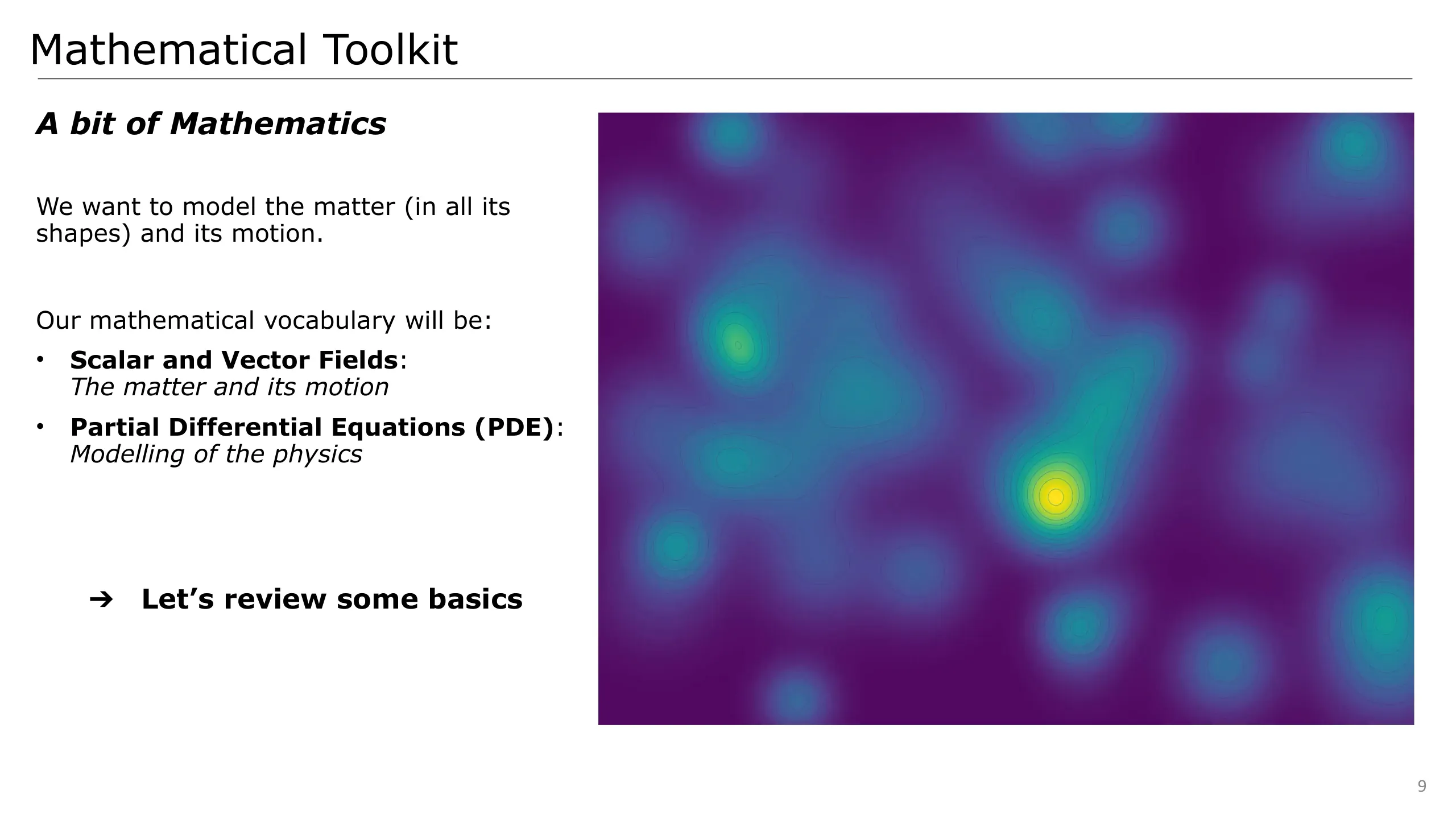
Represent the information on the matter like its density or its velocity: with fields (i.e. functions in space) like this one.

Describe how it moves: with partial differential equations relating time and spatial derivatives

Just to make sure everyone has the theoretical components for this part, we will quickly cover these tools

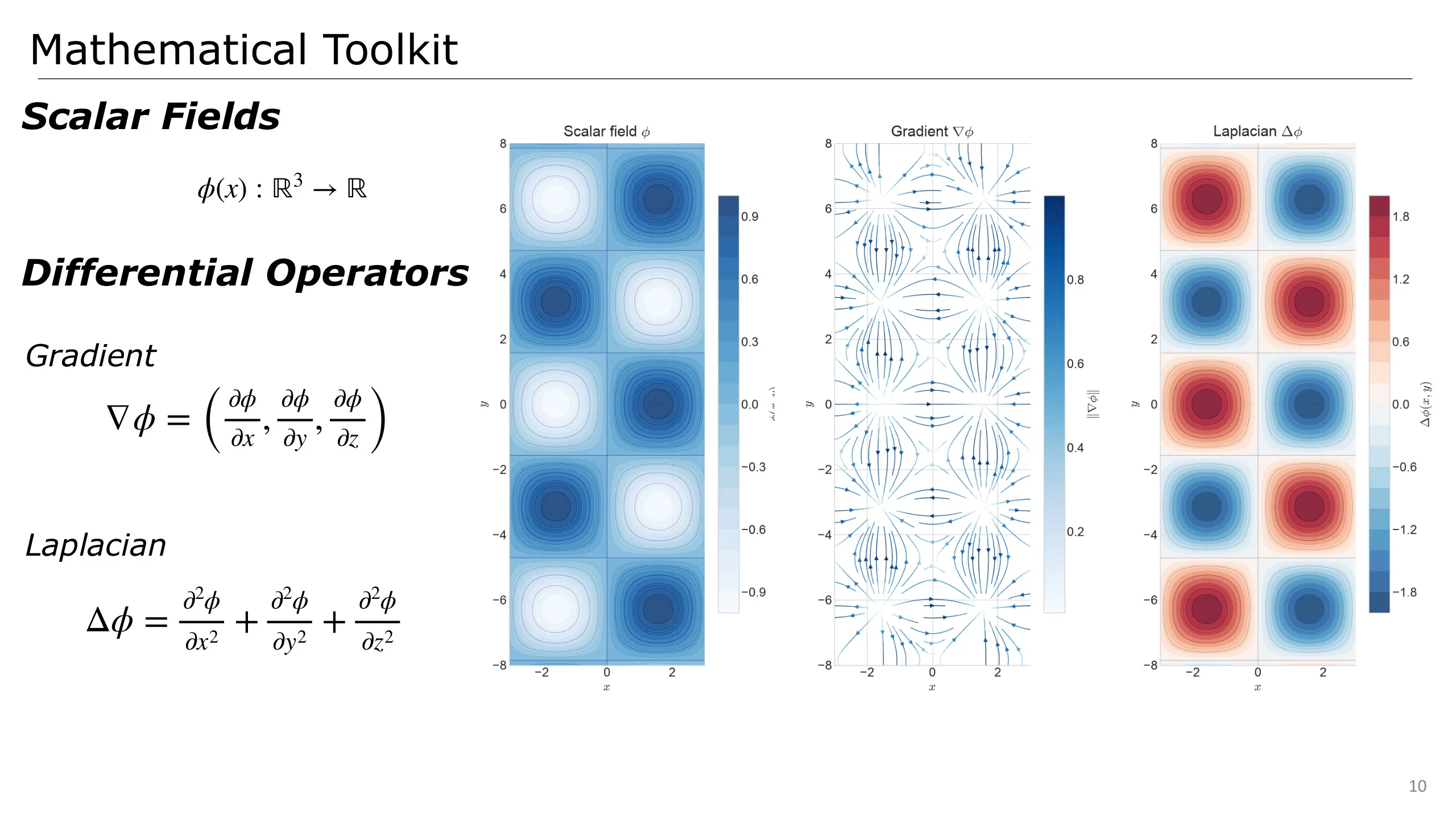
Scalar fields are functions taking a point in space and providing a scalar quantity at this point.

They can be used to represent the matter, or any other scalar quantities like energy.

To study their change in space, we can use the two differential operators:

- Gradient: Returns all partial derivatives in space and describes how the scalar field increases and in which direction

- Laplacian: the sum of second partial derivatives in space. It measures how a value differs to the mean of its neighbourhood.

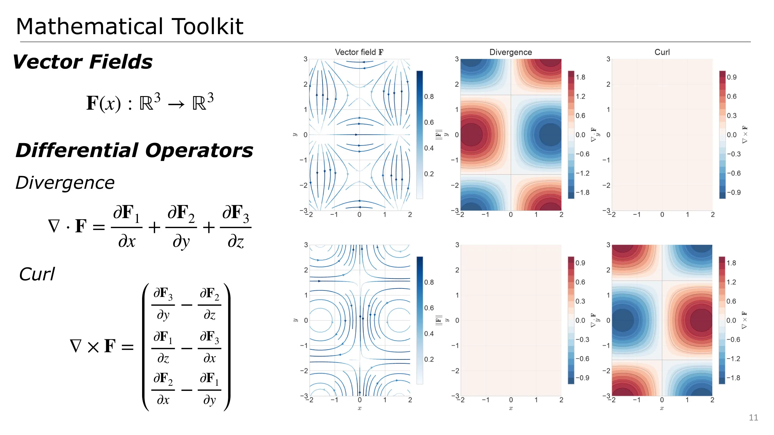
In fluid dynamics we will need to consider forces or velocity that vary in space which define a vector field: a function that associates a vector in 3D space.

They have interesting properties that can be studied from their change in space:

- The divergence describes the local flux: it indicates where quantity concentrates (in sinks) or becomes sparse (in sources). As we can see on the right, this is illustrated with matter converging or diverging at a specific point.

- The curl describes how much the vector field rotates around a point.

We chose here to show two fields with zero/non-zero divergence and curl to highlight the meaning of these operators

Now that we know how to describe spatial information, we must describe how they change over time.

This is achieved with the help of conservation laws and forces.

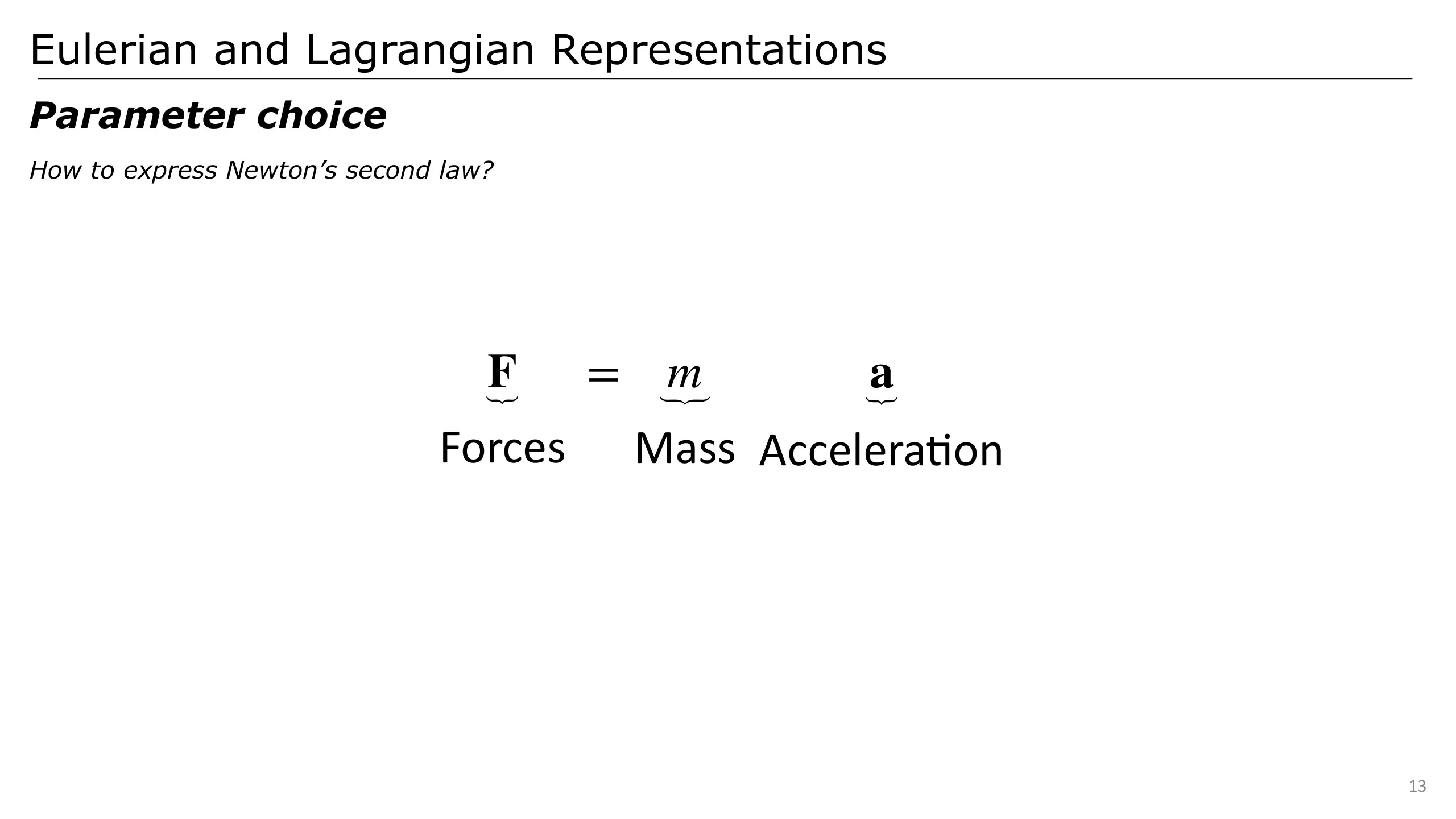
A good starting point is the momentum equation. It relates mass and acceleration to net forces which will lay the basis to model our fluid.

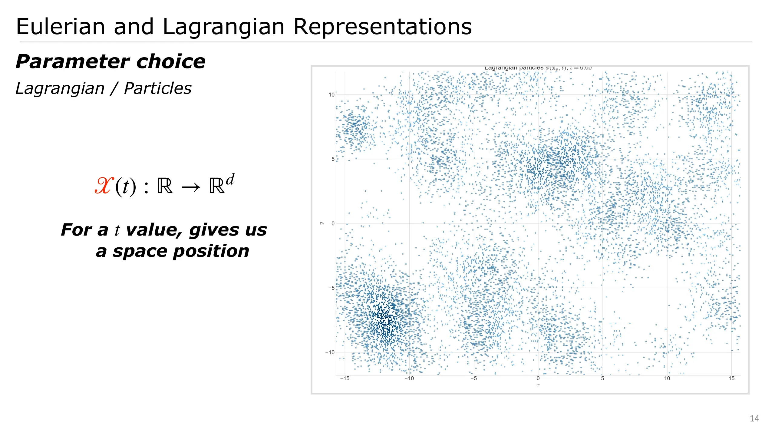
We may first focus on the acceleration, which is the time derivative of velocity. For that, we can first consider a set of particles, which are just moving points.

Here I’m representing these moving particles, that move across space while advancing in time.

To actually represent them in a mathematical language, we have to define a function that, at each time value, gives us the position of the particle.

We also have to indicate which particle we are talking about. For that, we can add another parameter which is the starting point of the particle

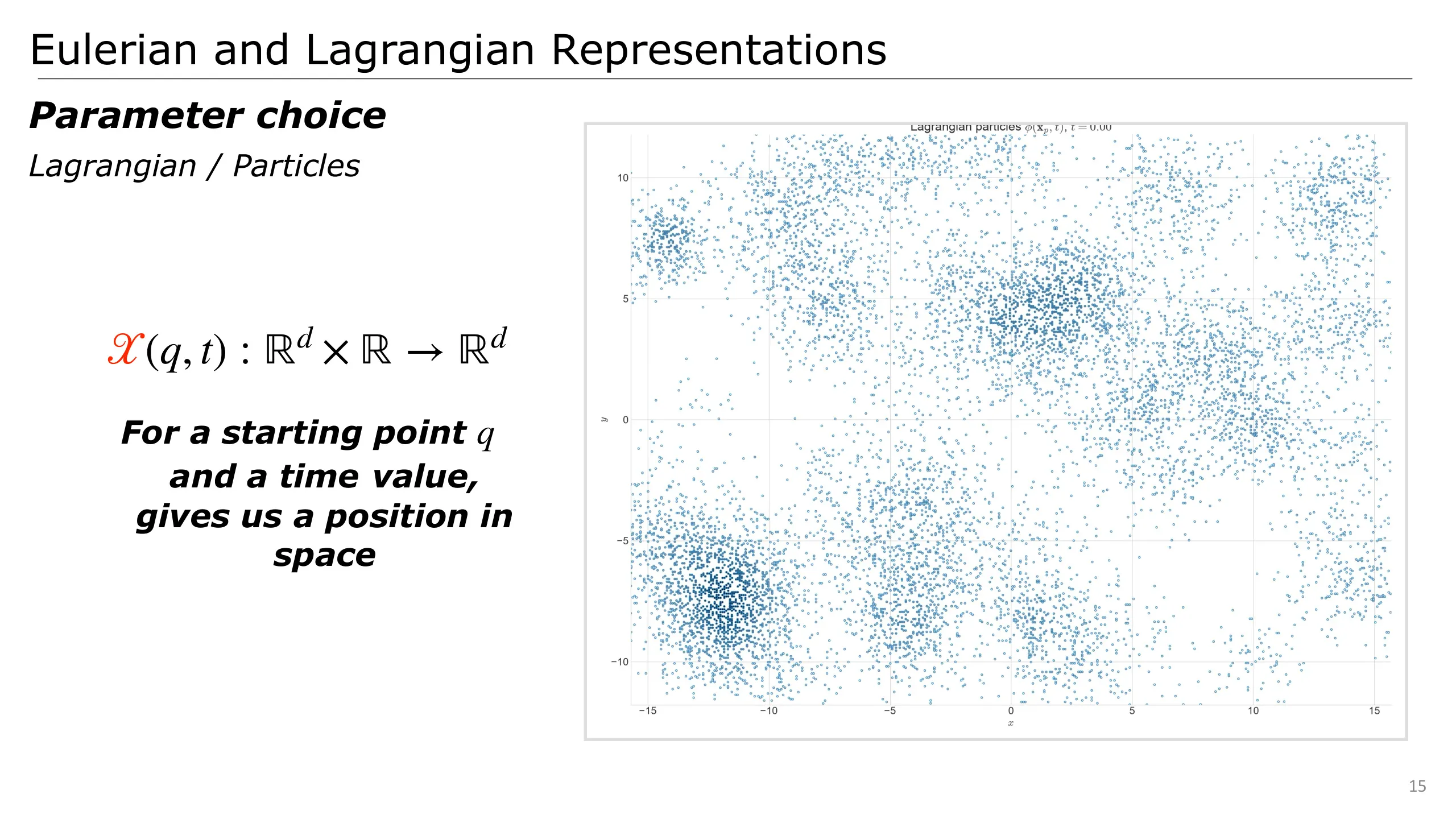
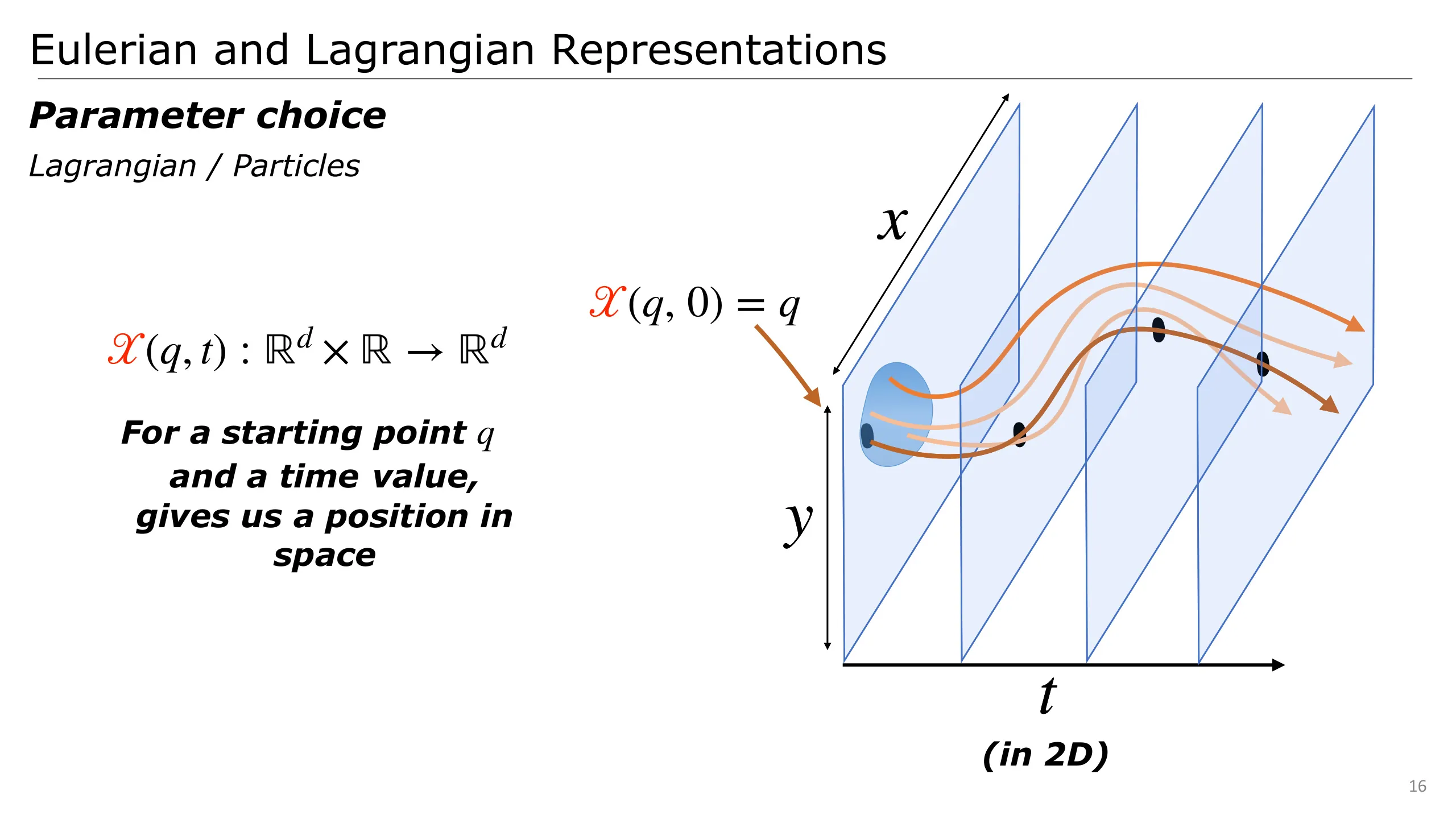
We also have to indicate which particle we are talking about. For that, we can add another parameter which is the starting point of the particle

In 2D, and for one particle, this function can be displayed in such way. We have the time in the bottom and the position of the particle on the other axis.

The first point is then the starting point.

This function then represents the trajectory of the particle over time.

Considering multiple particles results in such plots.

This way of representing the position in space is called a Lagrangian point of view and it is very handy to express our motion relation.

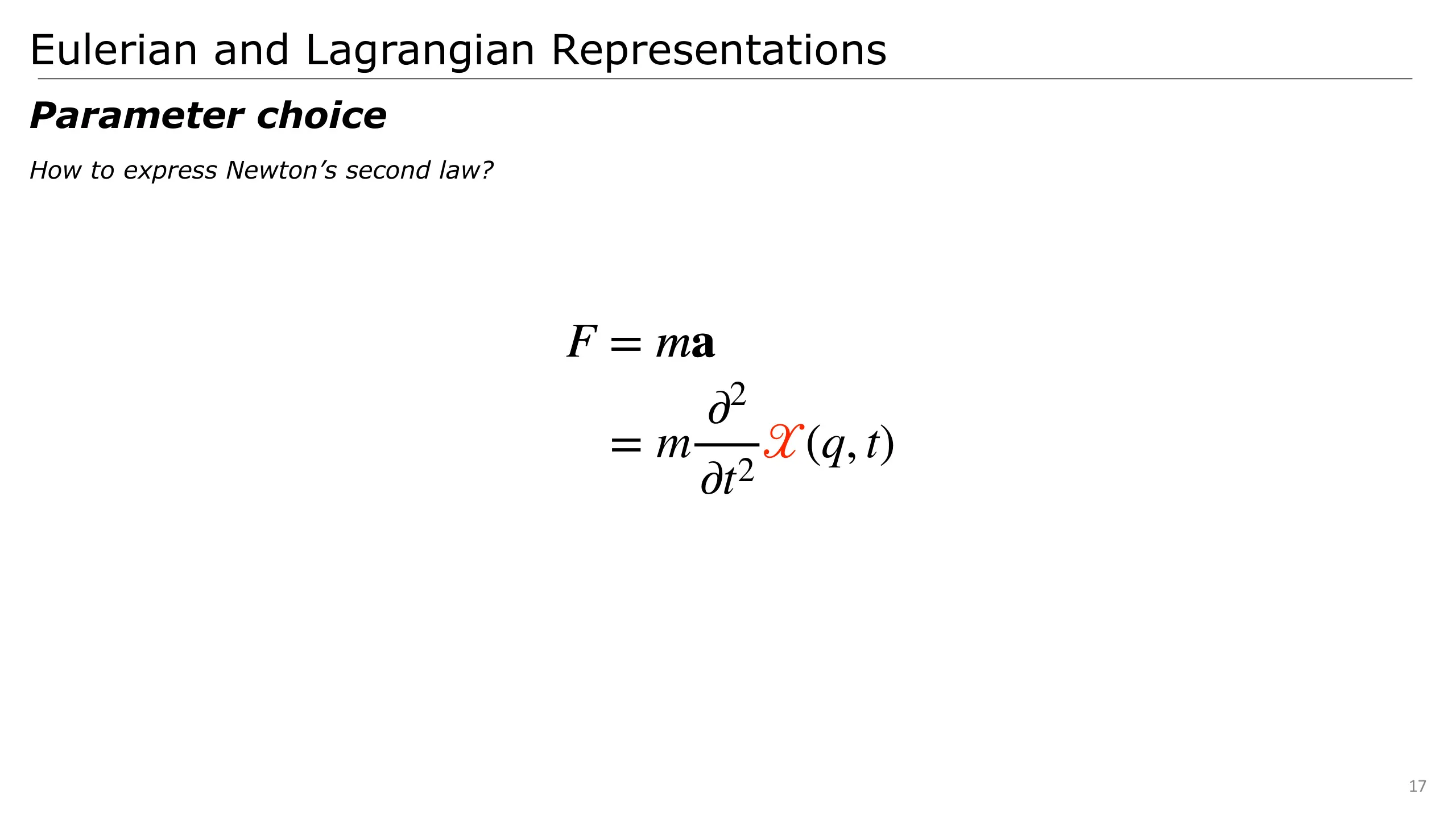
Coming back to our motion relation, we now want to express acceleration.

With Lagrangian particles, it is very easy: we can directly differentiate the trajectory two times in time.

This point of view may however often be not enough.

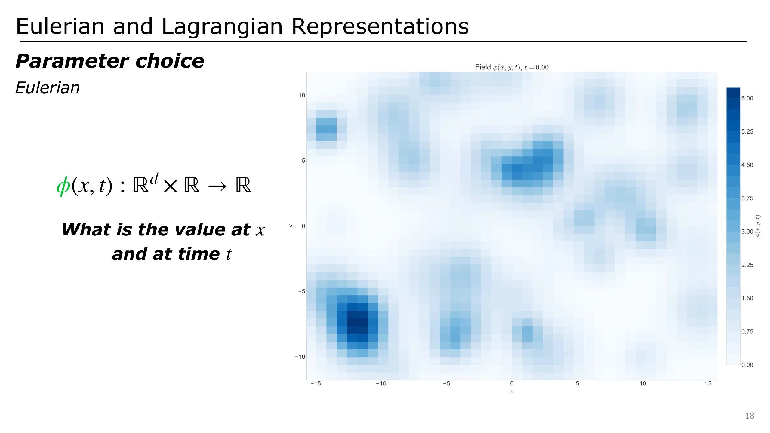
In contrast with particles, it may be interesting to study how the matter changes in time at fixed location.

For instance, if we look at a flowing river, and consider fixed points in space like in a grid. You can ask how the fluid changes at these fixed locations.

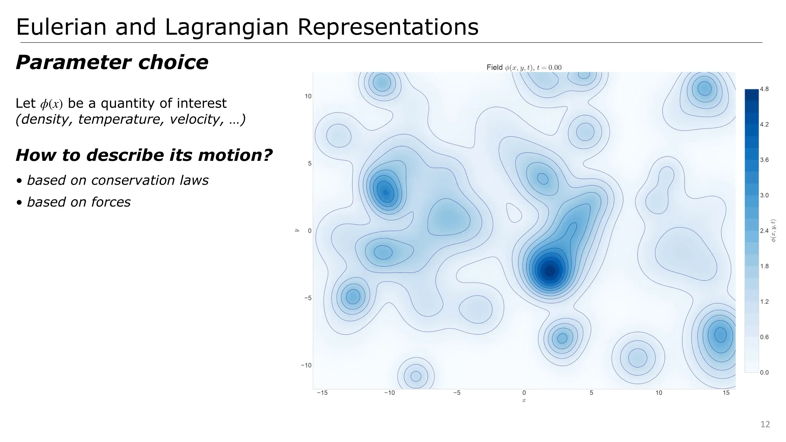
For that, we can define another parameter choice, called Eulerian point of view, that gives us the quantity of interest at a fixed location x and at a time t.

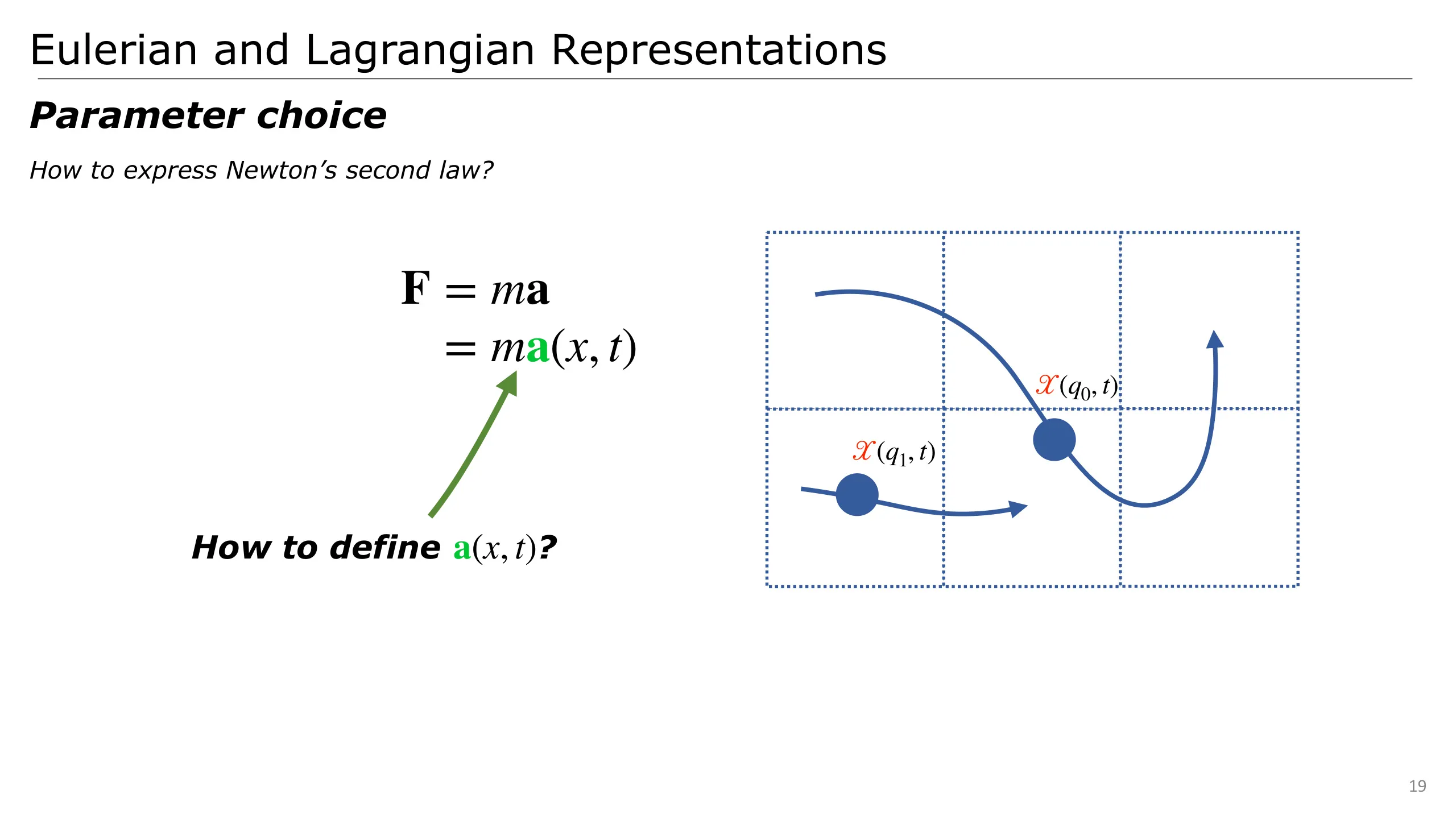
If we again come back to our equation of motion, we can consider an Eulerian acceleration field, i.e. how matter is moving across the grid.

Since the acceleration is a very Lagrangian quantity, we have to define it in an Eulerian point of view.

This means, how to consider the motion of the particles in our Eulerian fixed coordinate point of view?

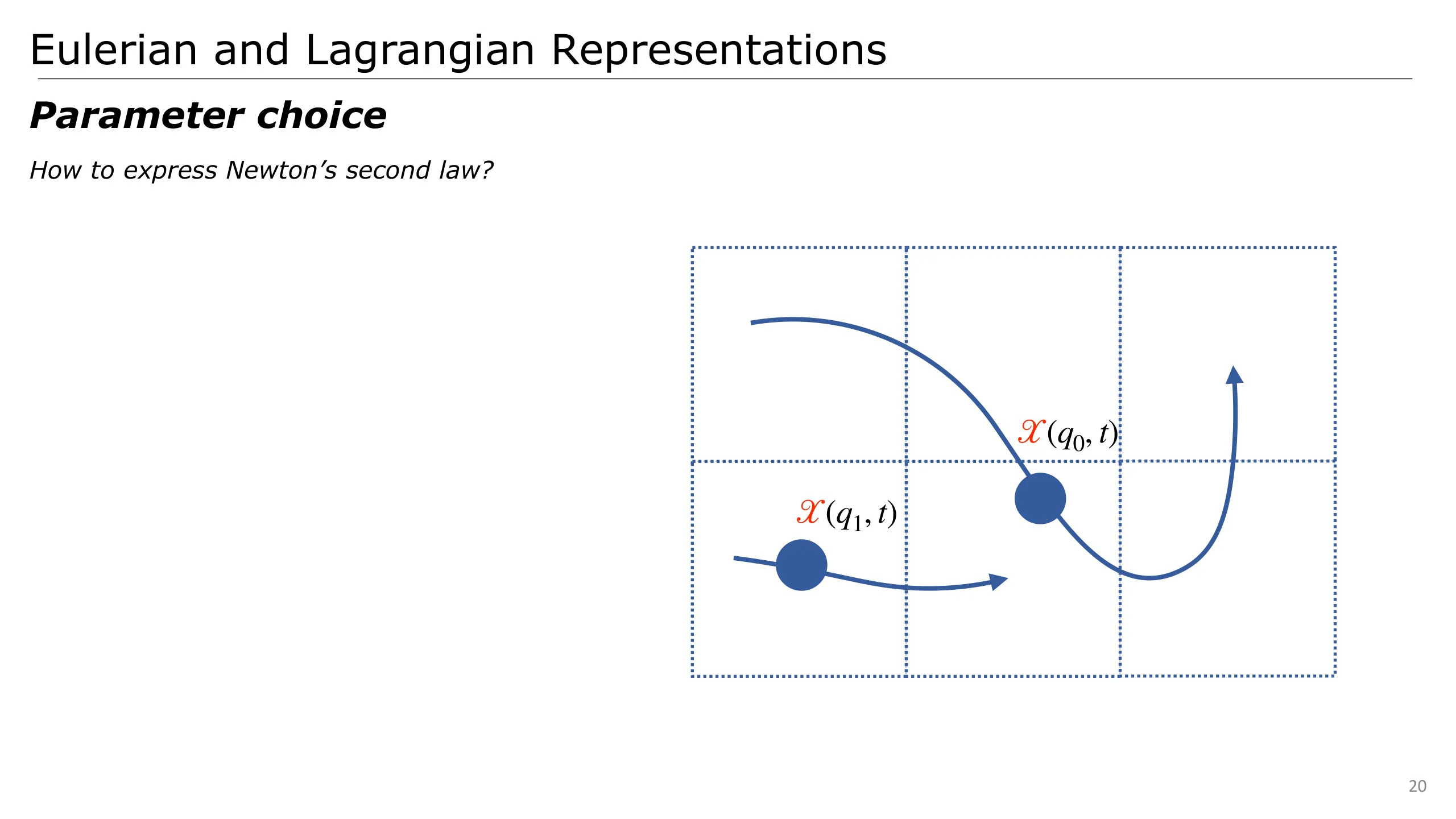
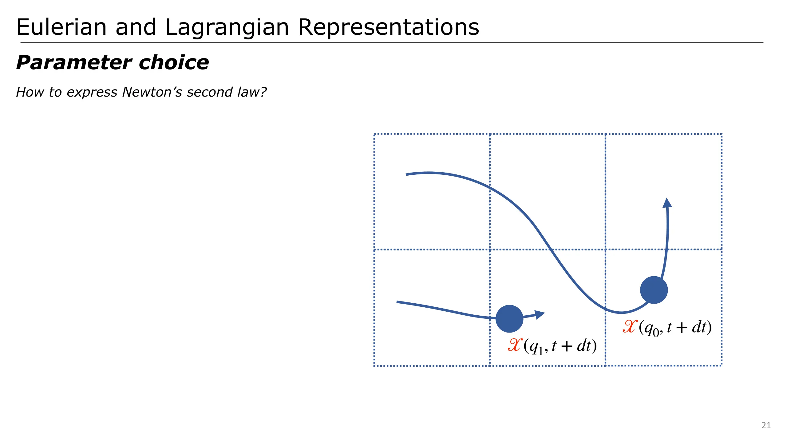
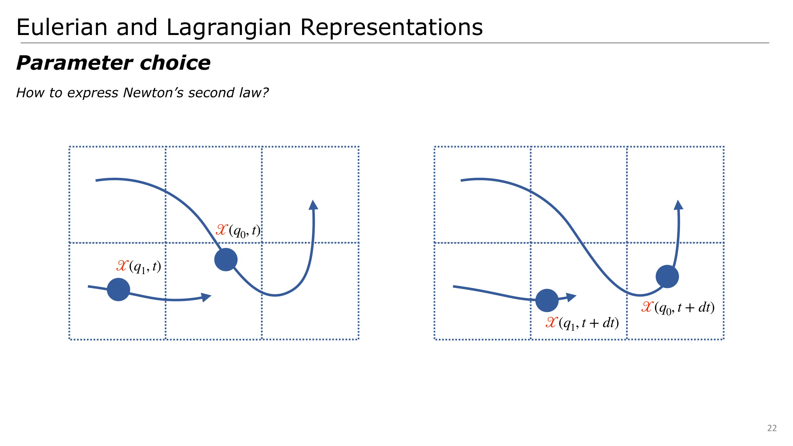
To see how, we may consider two consecutive time steps, two particles’ paths and an Eulerian pov represented as a grid.

Here is the time step dt later

And now we can look at them side by side

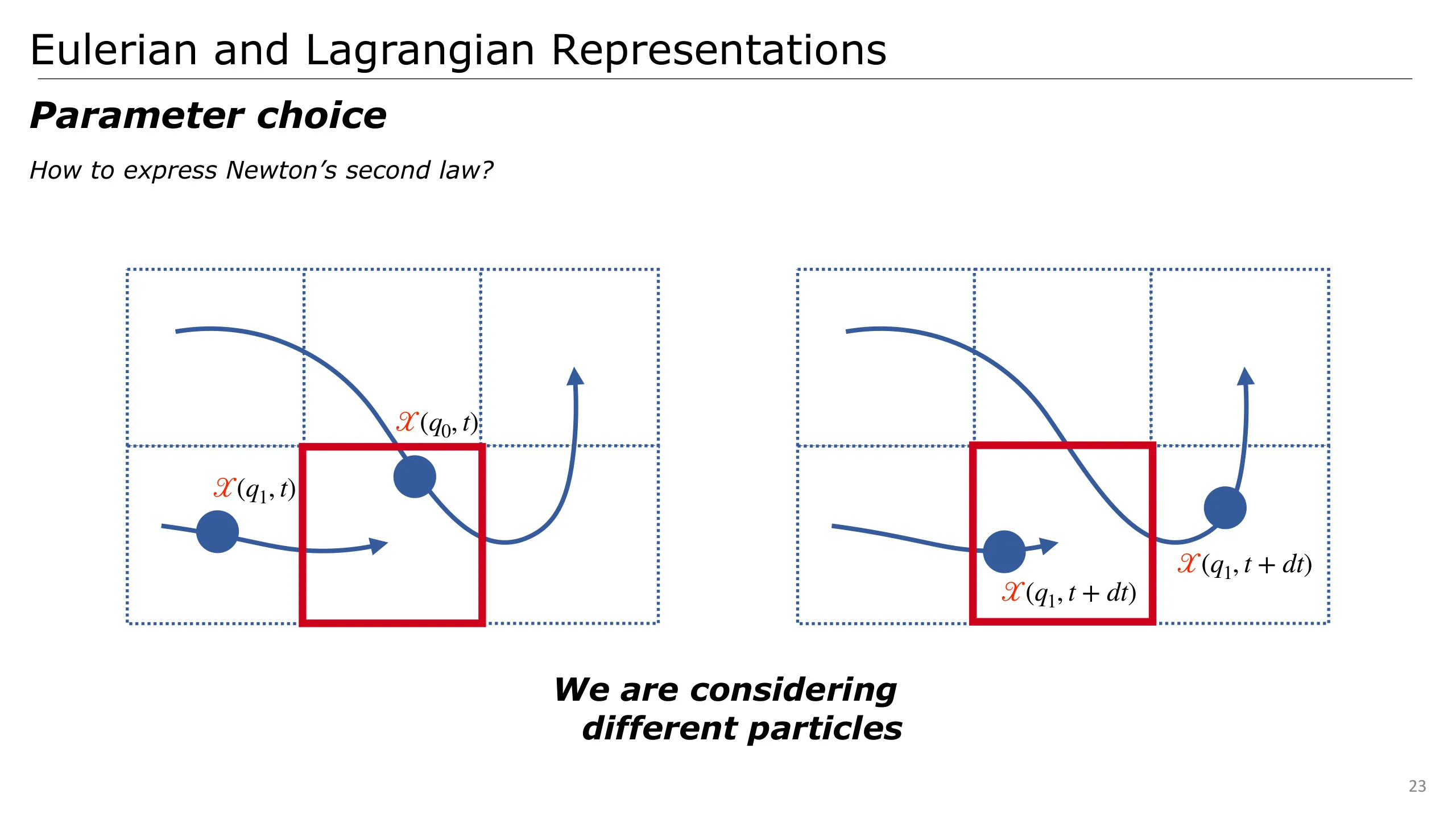
As we can see here, if we consider the red cell, at time t, it is linked with the Lagrangian particle coming from q0.

However, at time t + dt, we are considering the Lagrangian particle coming from q1.

Thus, the acceleration must take into account this information.

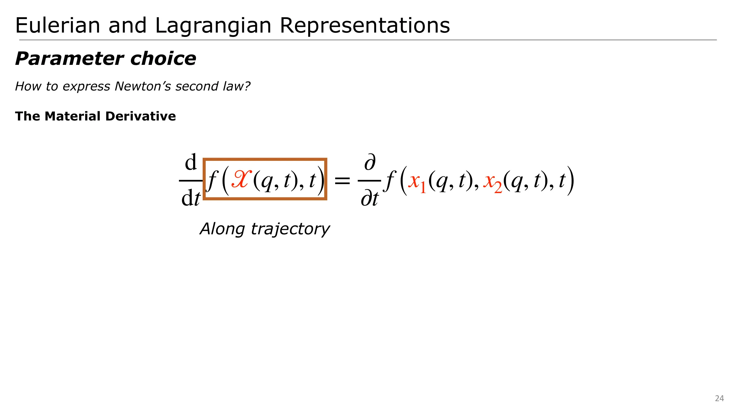
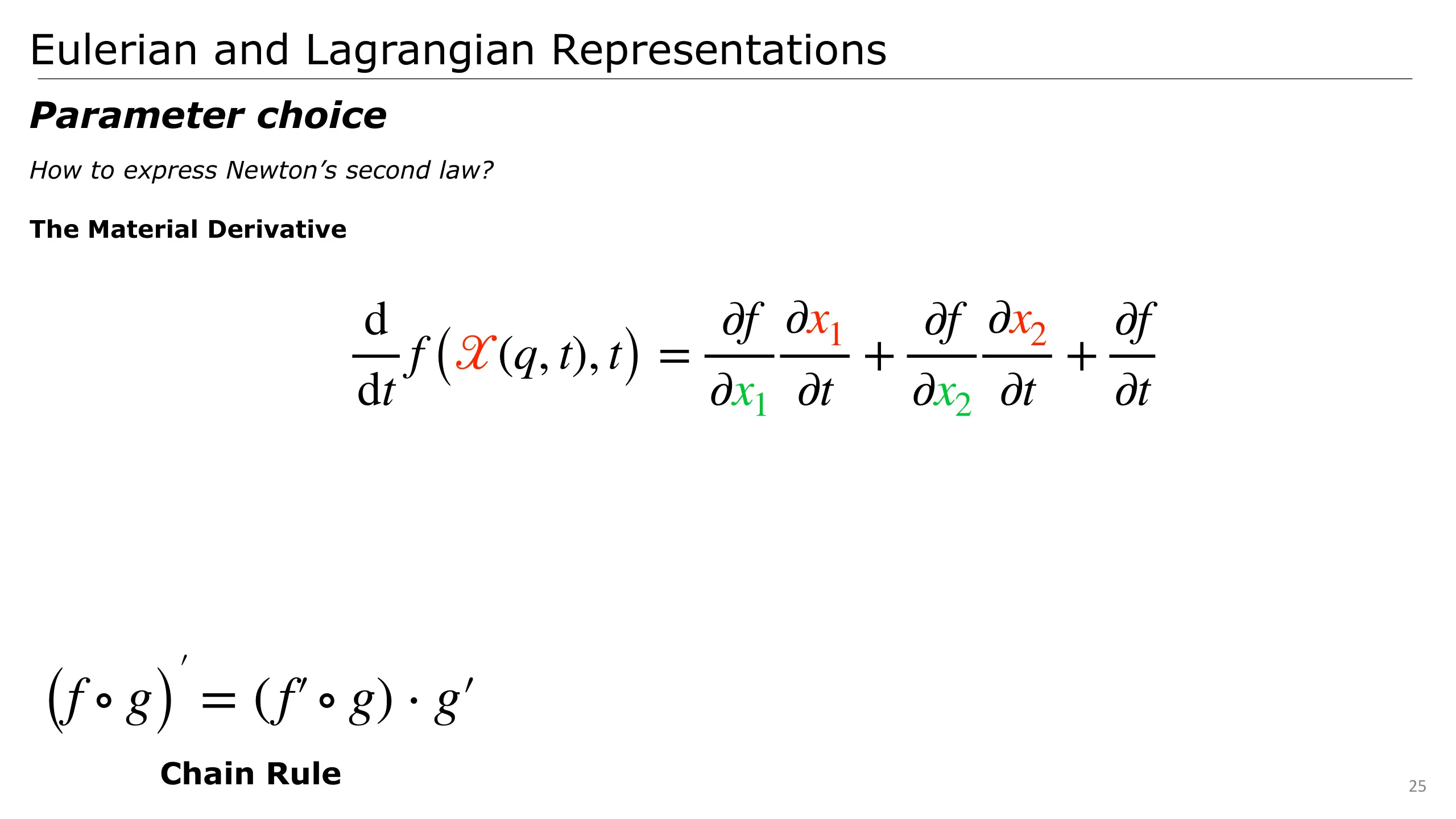
This can be made by studying the rate of change of a quantity in space (an Eulerian pov) along a Lagrangian trajectory (the path of a Lagrangian coordinate)

To better understand this development, we can unroll the Lagrangian coordinates (here in 2D).

We can develop our expression by applying the chain rule to each argument of our function

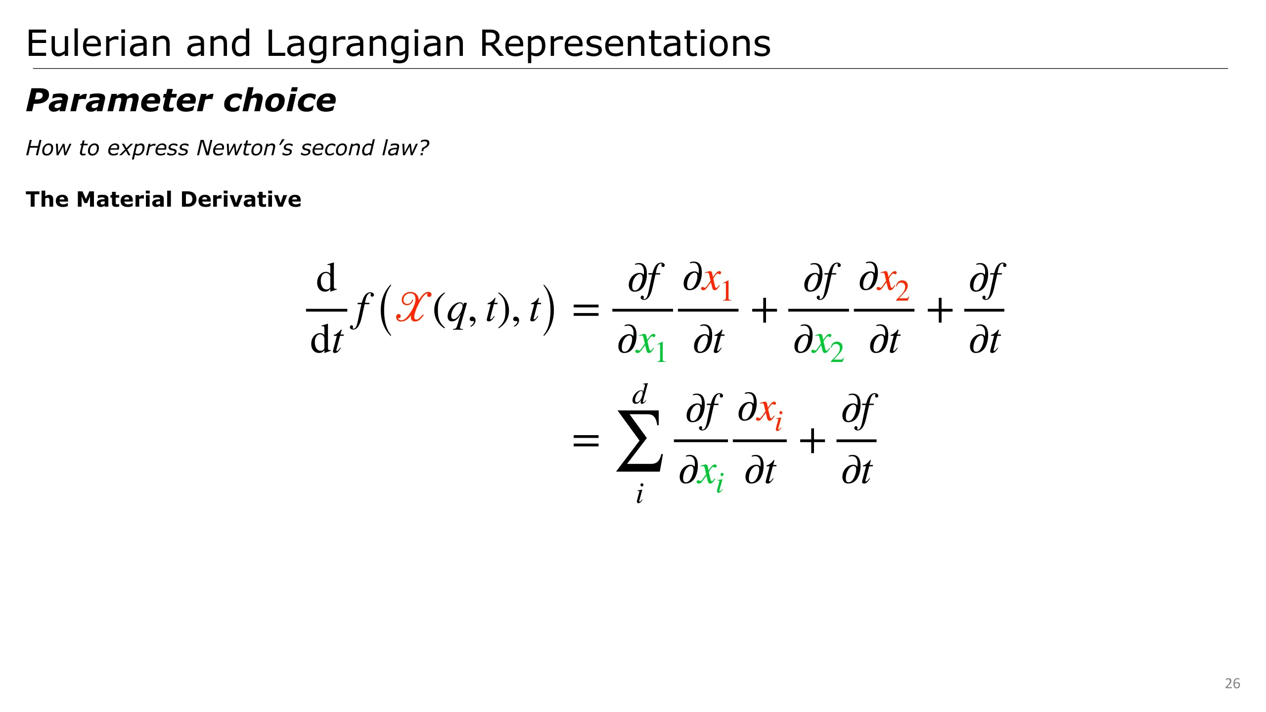
…that we can compact by summing all coordinates derivatives…

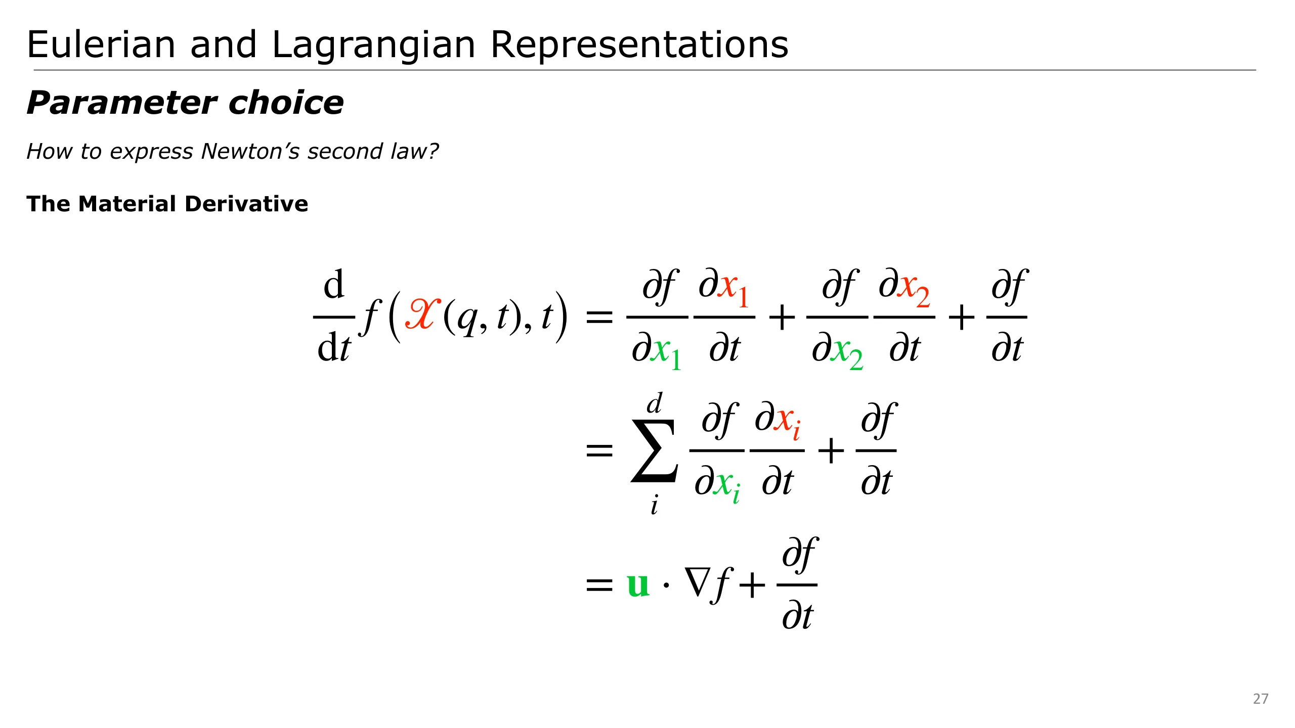
… and identify that they can be seen as the dot product between the velocity of the fluid and the gradient of the potential.

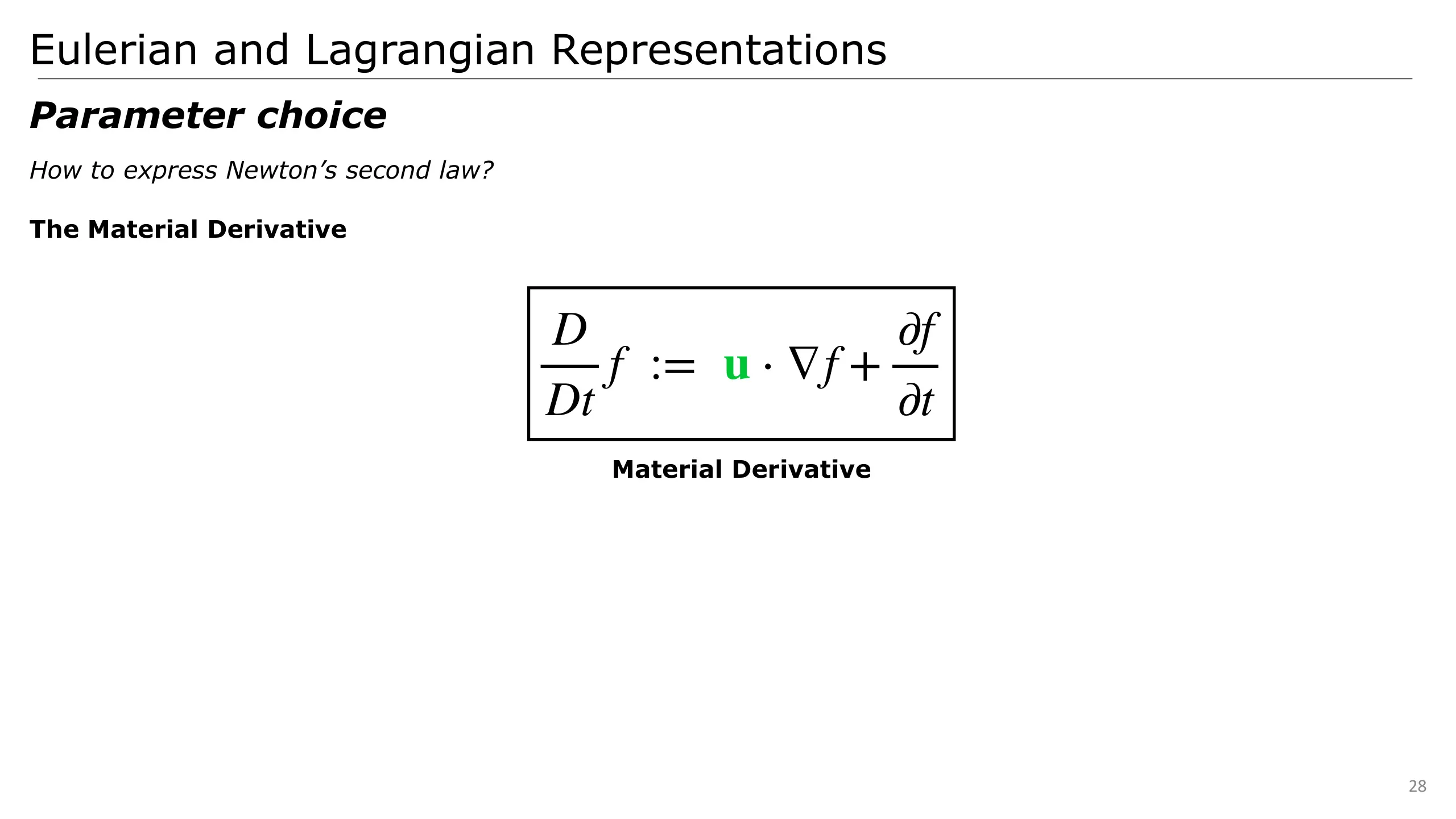
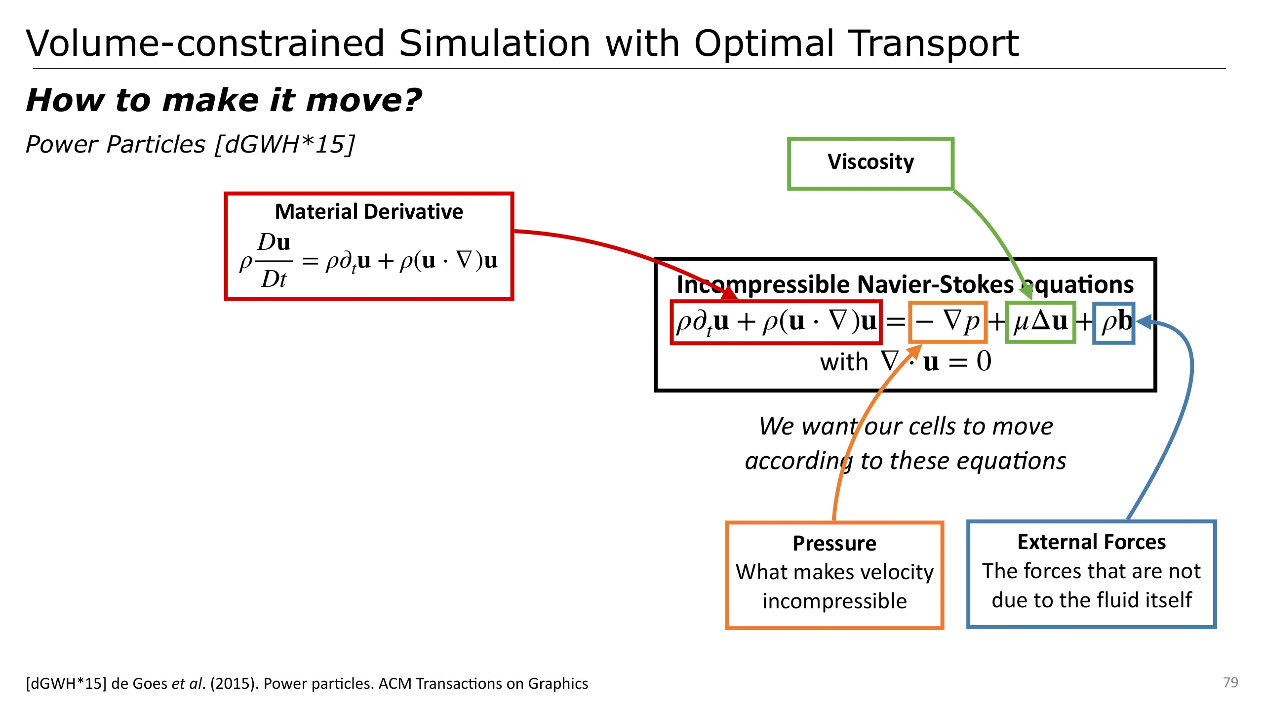
This result allows us to express a Lagrangian quantity in an Eulerian pov.
It is referred to as the Material Derivative and denoted capital D over capital Dt to avoid confusion with standard derivative notations.

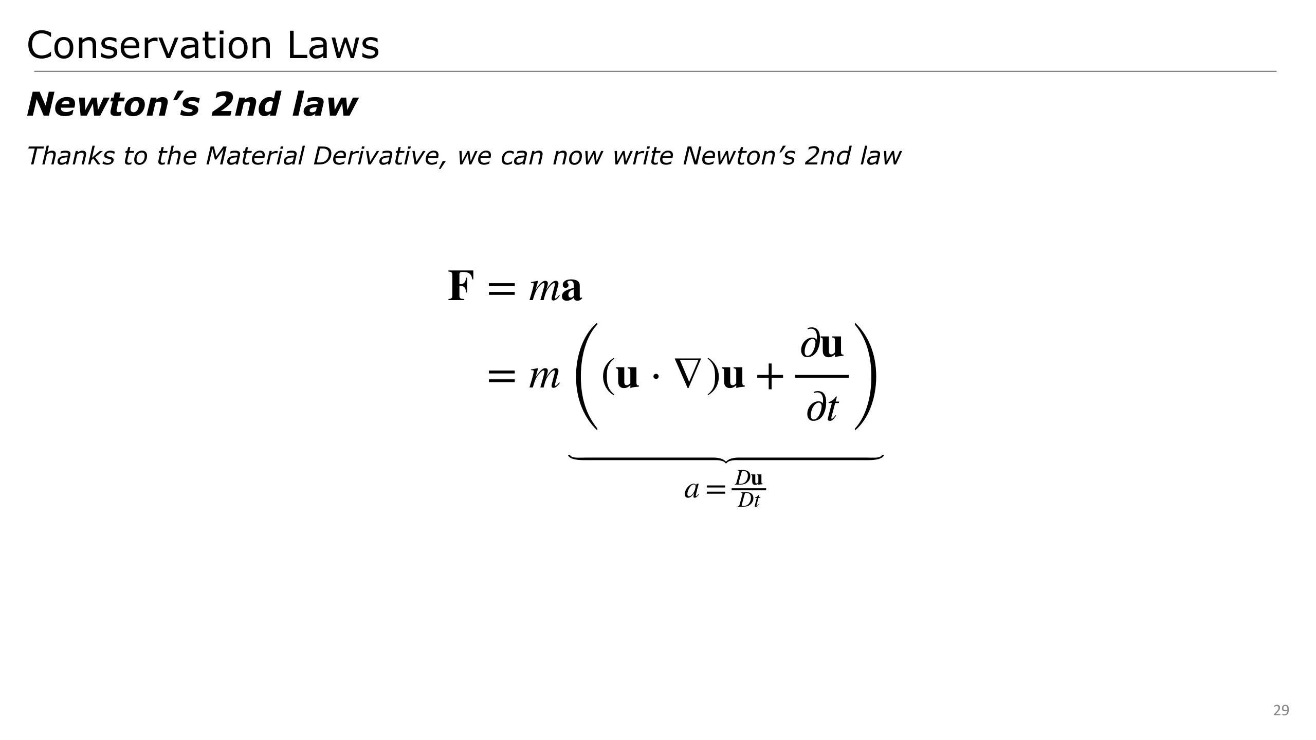
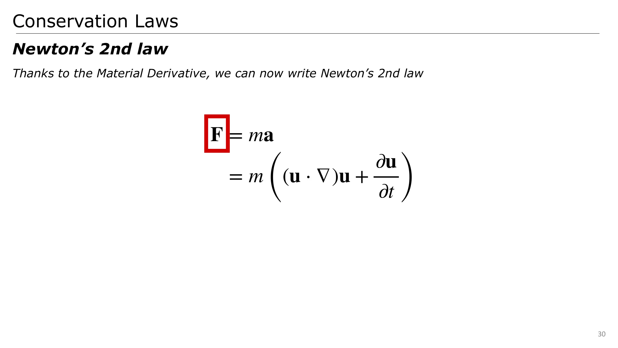
Based on these developments, we can now express Newton’s 2nd law relating Forces to mass and acceleration.

Now that we have one part of this law, we may study what is inside the force term.

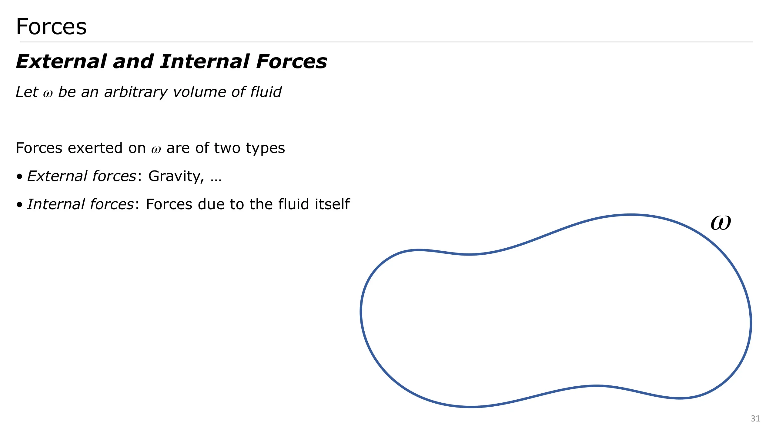
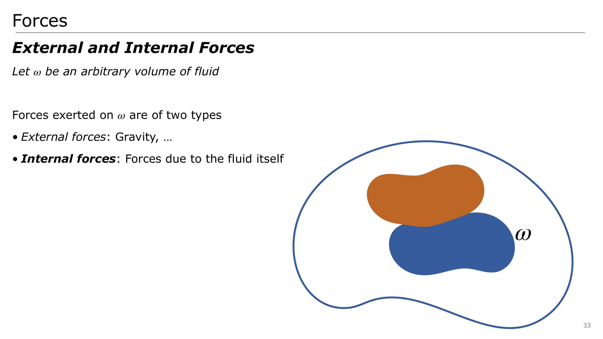
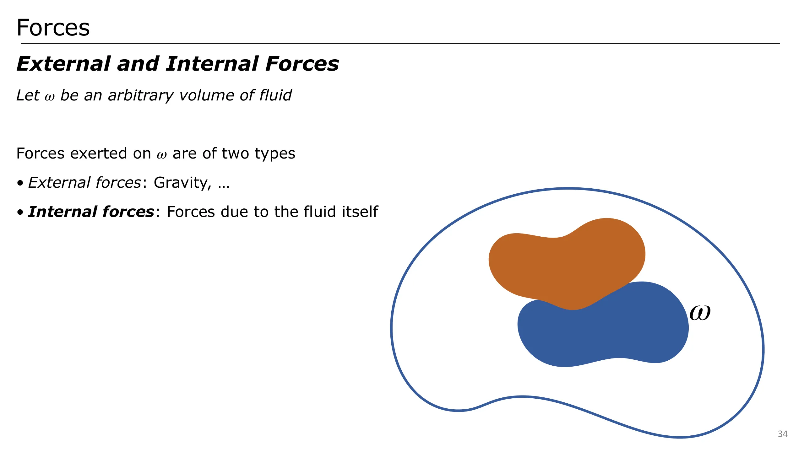
Two types of forces can be considered for the motion of our fluid: external and internal forces

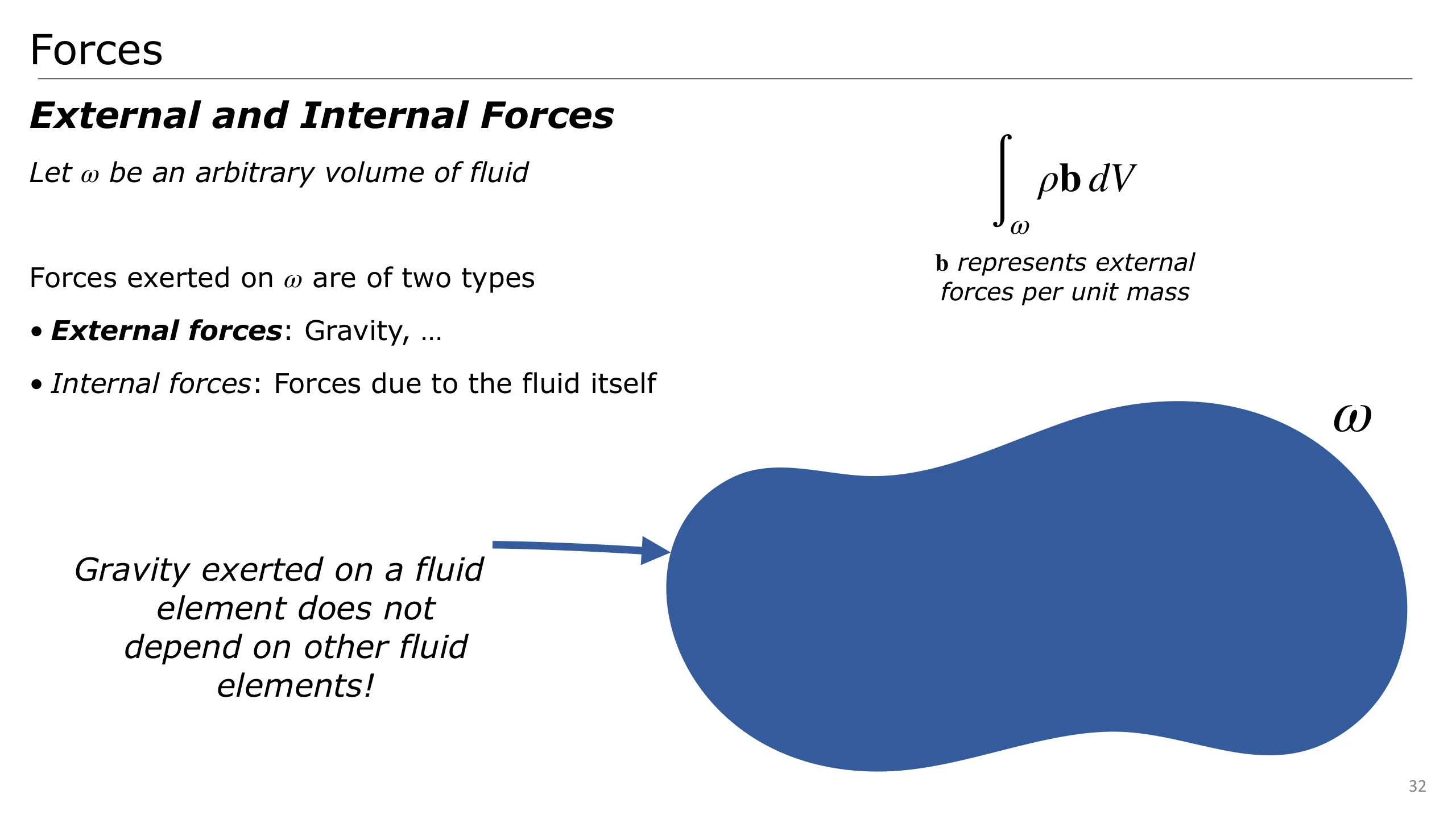
External forces are composed of forces like gravity or electromagnetic forces, they are not due to the fluid itself.

If we consider an elementary volume of fluid omega in blue,

If you’re an atom of fluid in this elementary volume, the gravity you feel does not depend on your neighbours!

They can then be collected all over the fluid volume as written in the upper right corner.

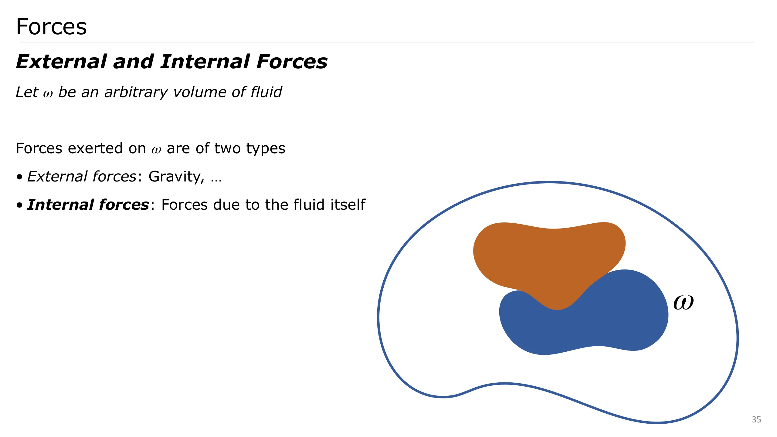
In contrast, internal forces are forces that the fluid exerts on itself.

To better understand this, we may consider that our elementary volume of fluid omega is a part of a larger fluid volume.

Our fluid element omega is then next to another one, that has motion too.

When this neighbour moves in omega’s direction, omega must move away to let the other pass

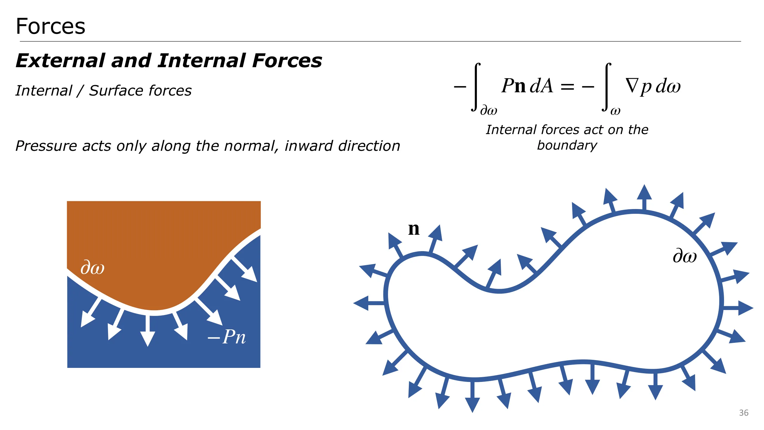
A first important internal force is the pressure. Pressure is the force pushing the fluid away to prevent matter from concentrating.

It acts inward along the normal, as illustrated on the left. The force of pressure due to the orange part onto the blue part is oriented *inside* the blue part and along the normal of its boundary.

It can then be represented as a volume force through the gradient of a potential.

In the next parts of this presentation, I will often qualify this force as what makes the fluid incompressible.

Viscosity is another important internal force.

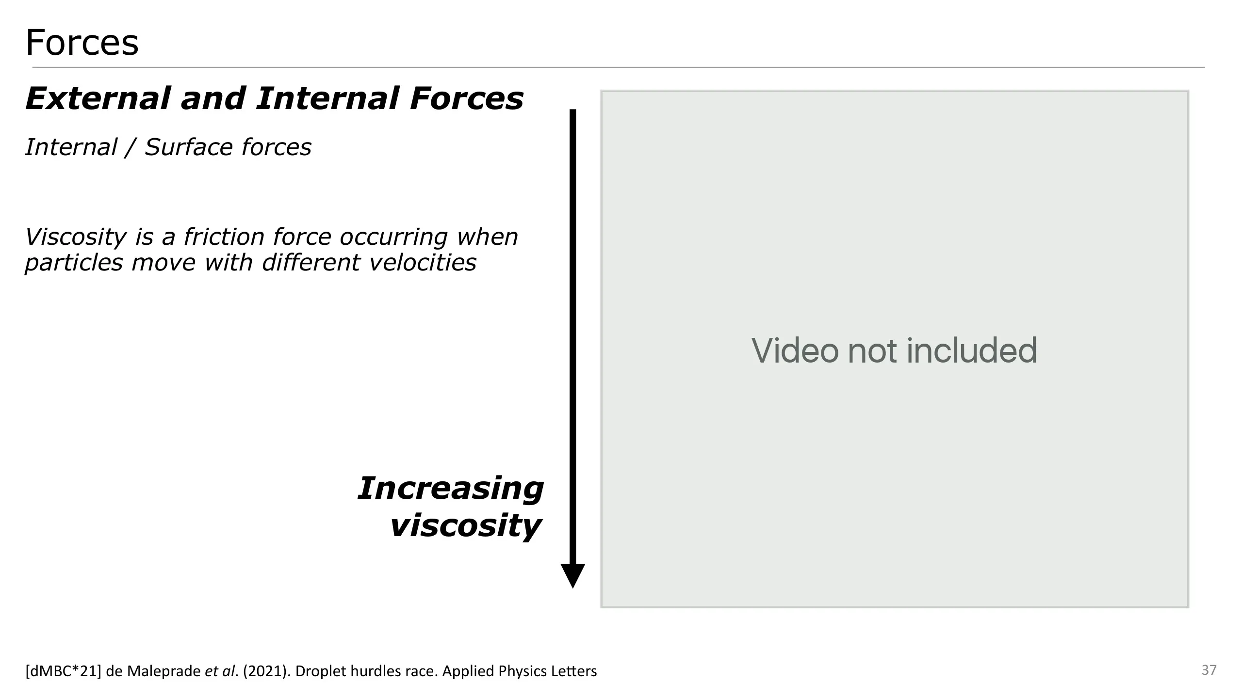
As we can see on this video, the most viscous fluid jiggles way less than the other.

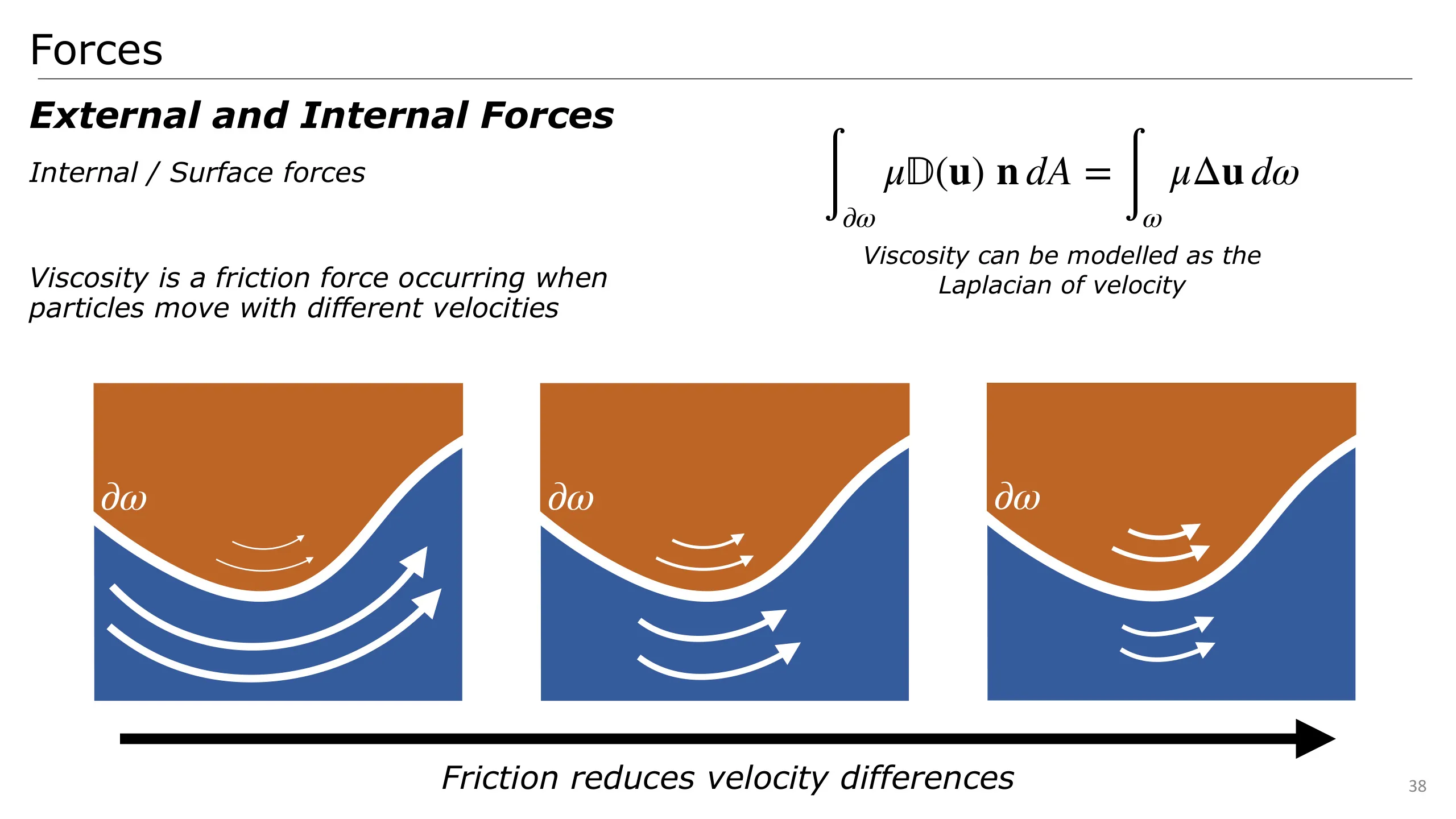
Inside the fluid, we can directly infer that velocities are more homogeneous when viscosity is higher.

Viscosity is a kind of friction inside the fluid between particles having different velocity.

On this schema, we can see two parts of the fluid moving in different directions. The viscosity will make velocity equal, smooth velocity difference.

It is then described by how the velocity changes across the fluid. One possible modelling is then through the laplacian of the velocity field.

We may now study one last law of conservation, in addition with Newton’s 2nd law.

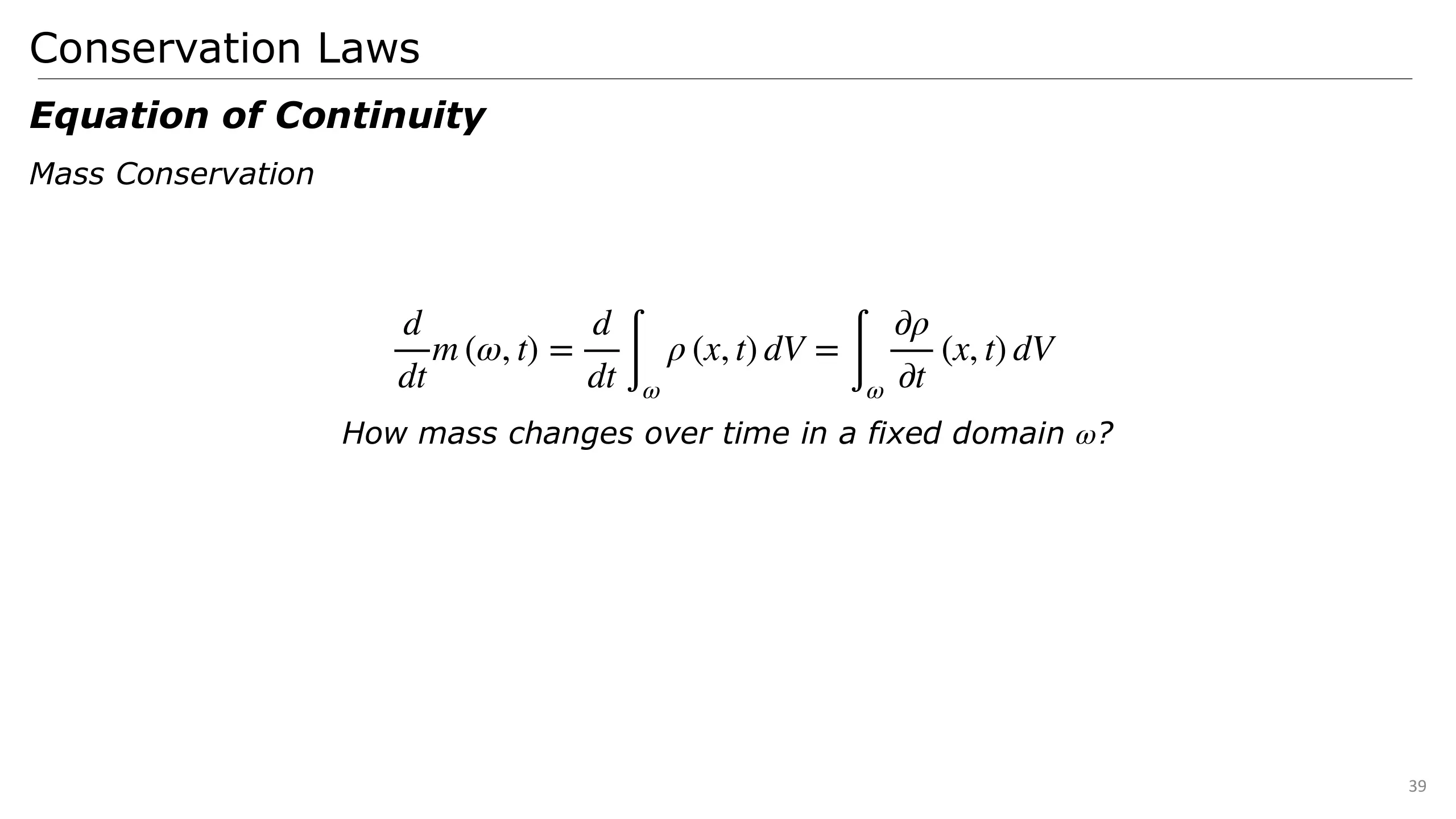
This important law describes how mass changes over time.

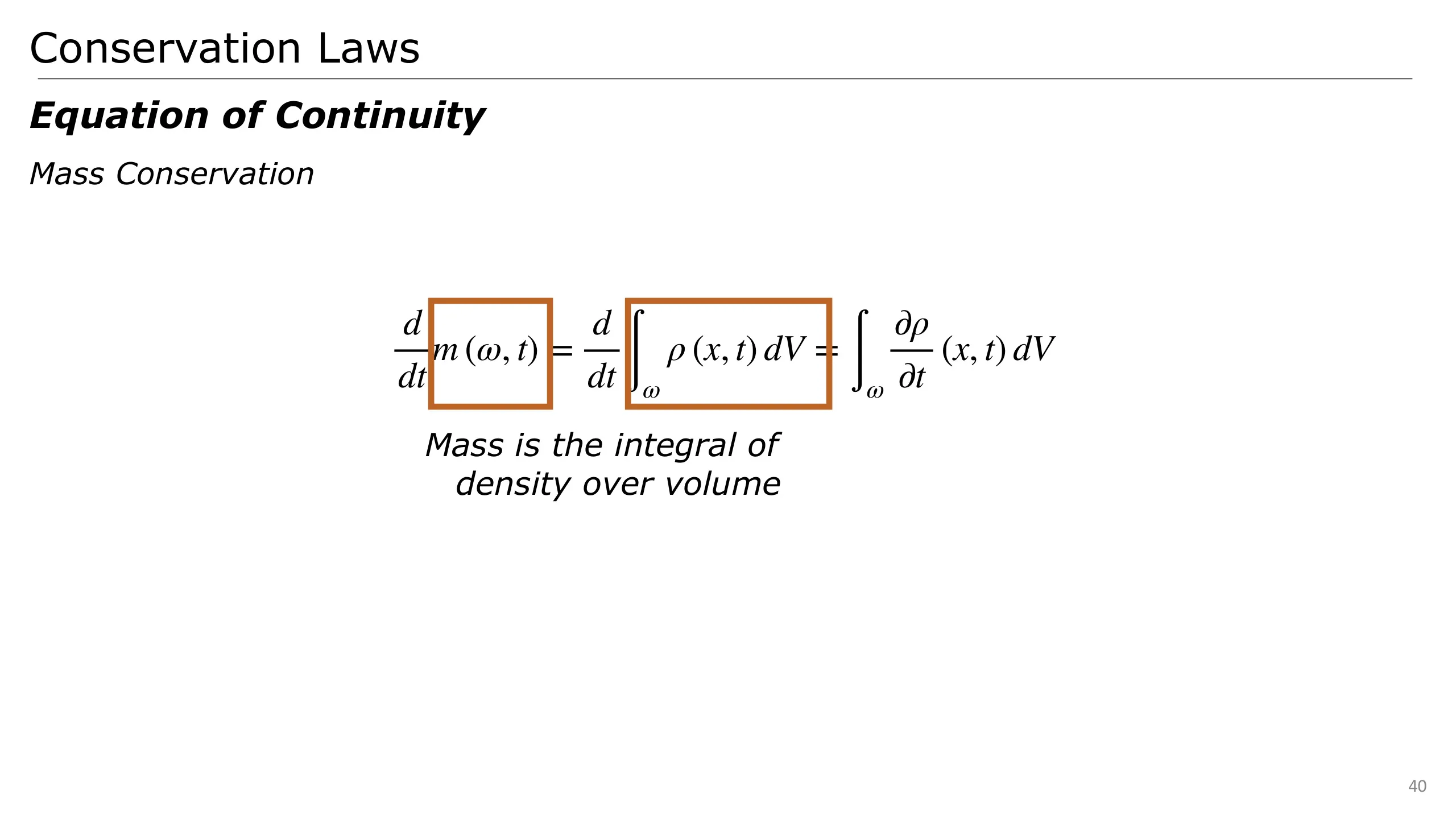
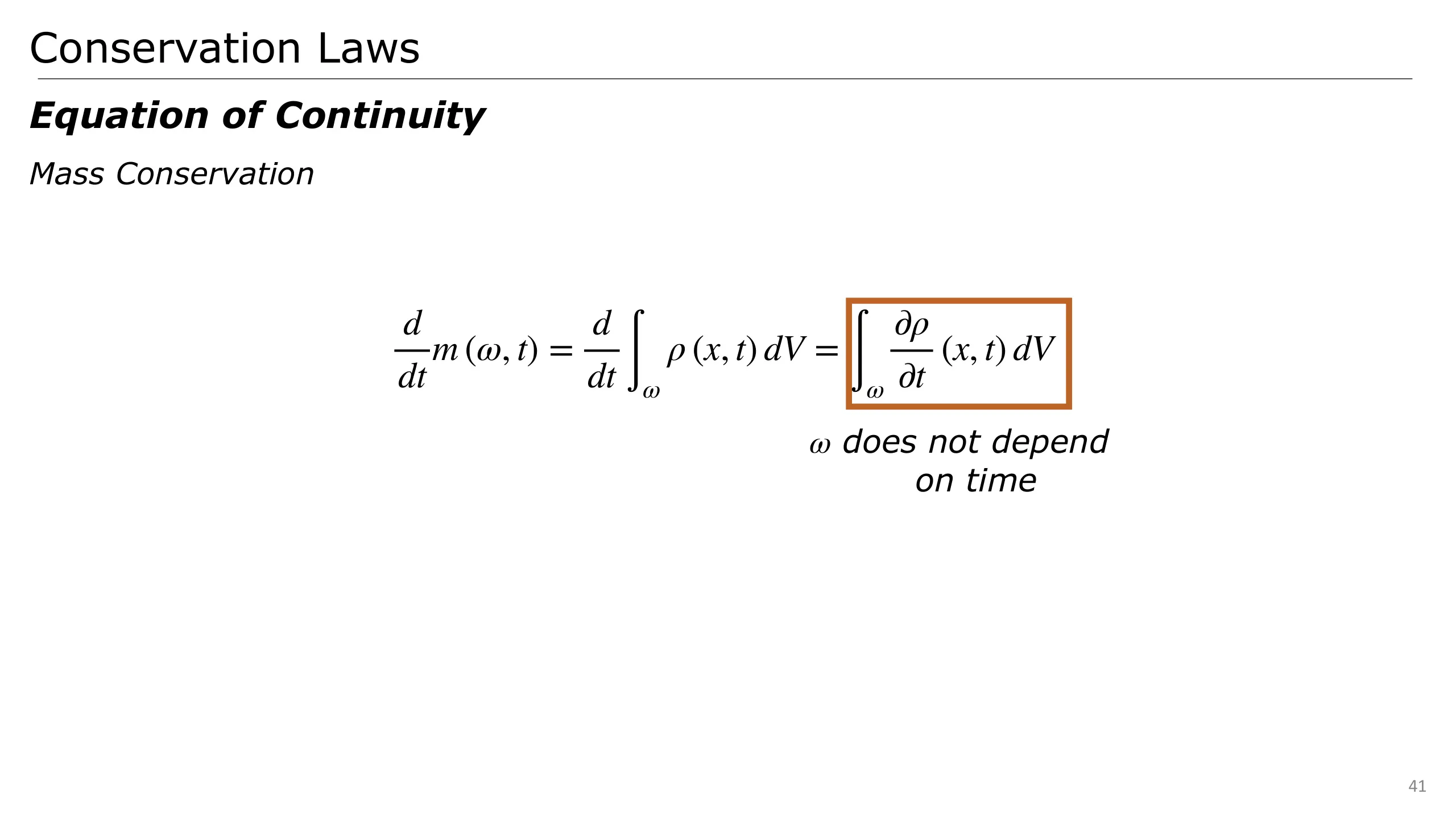
So we have the mass, which is equal to the integral of the density over the volume.

We want to know how this quantity changes across a fixed volume so we can push the derivative inside the integral.

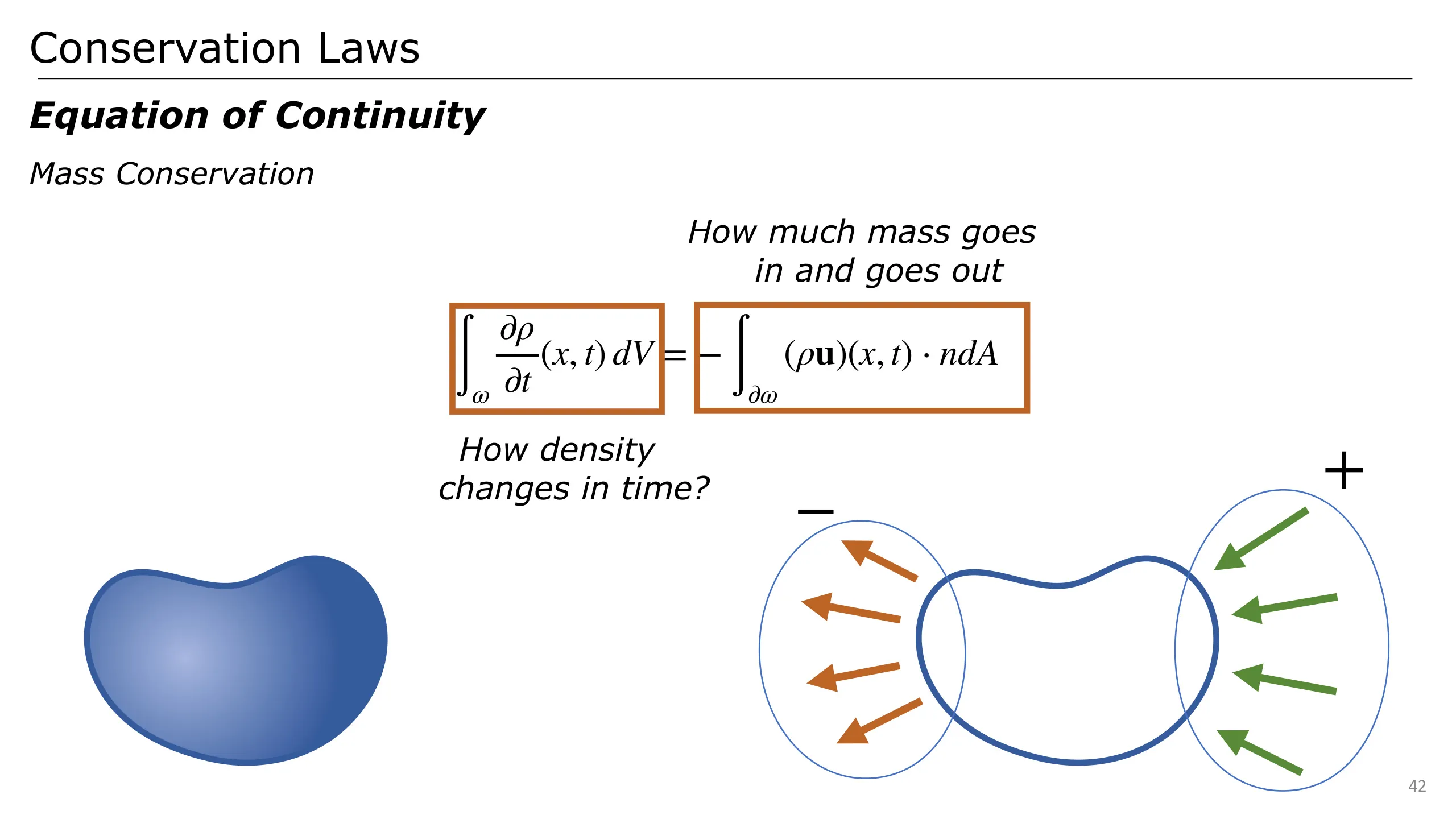
We know that density cannot disappear, so if the integral of density over a volume changes, it means that some went in or away.

We can formulate this equality with the boundary integral of the rate at which mass is crossing the boundary of omega. This is the flux of matter over the boundary of omega.

We push the boundary integral on the lhs

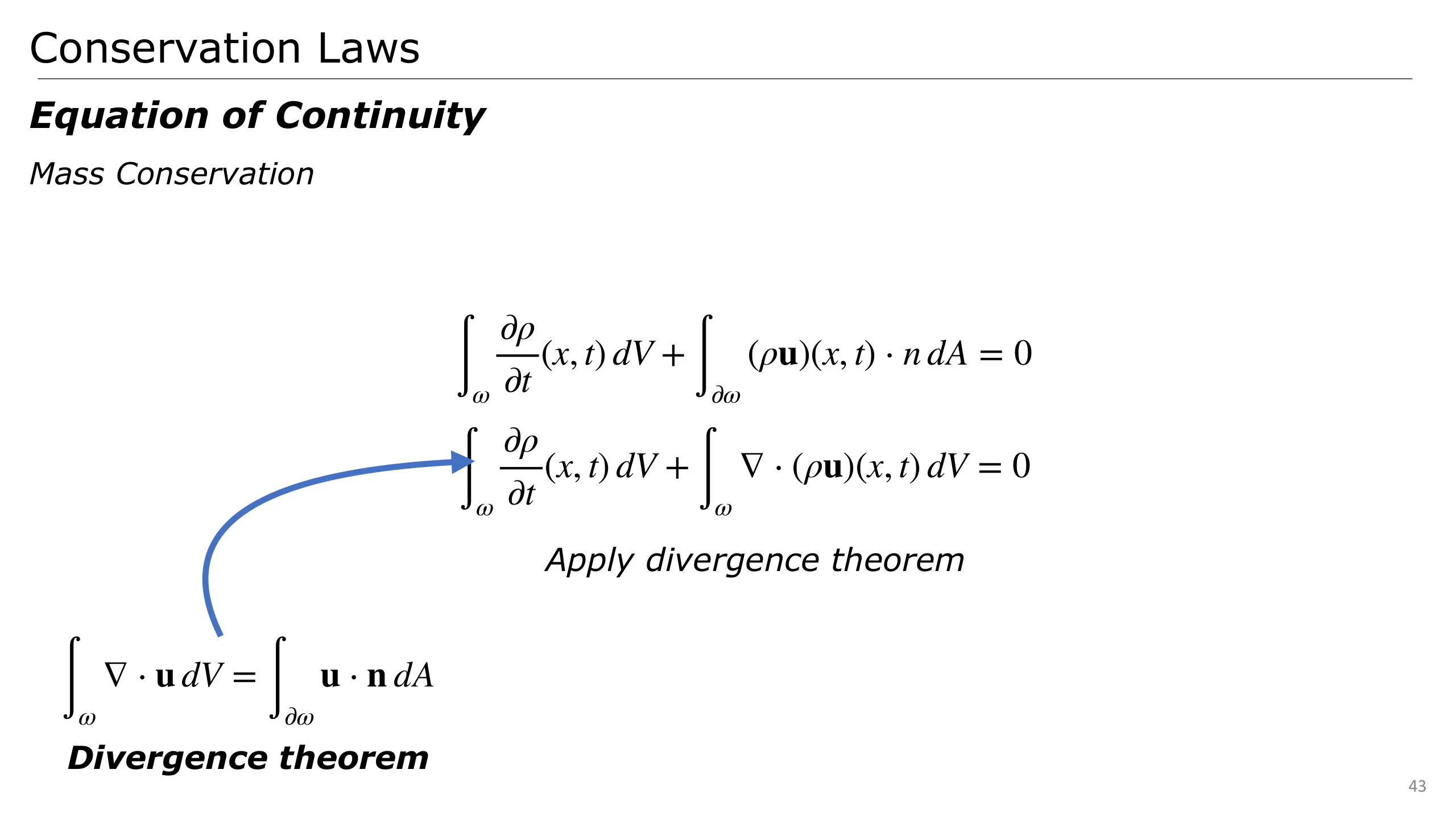
Apply divergence theorem on it.

This allows to express the boundary integral to a volume integral of its divergence.

By grouping the integral we obtain a single volume integral.

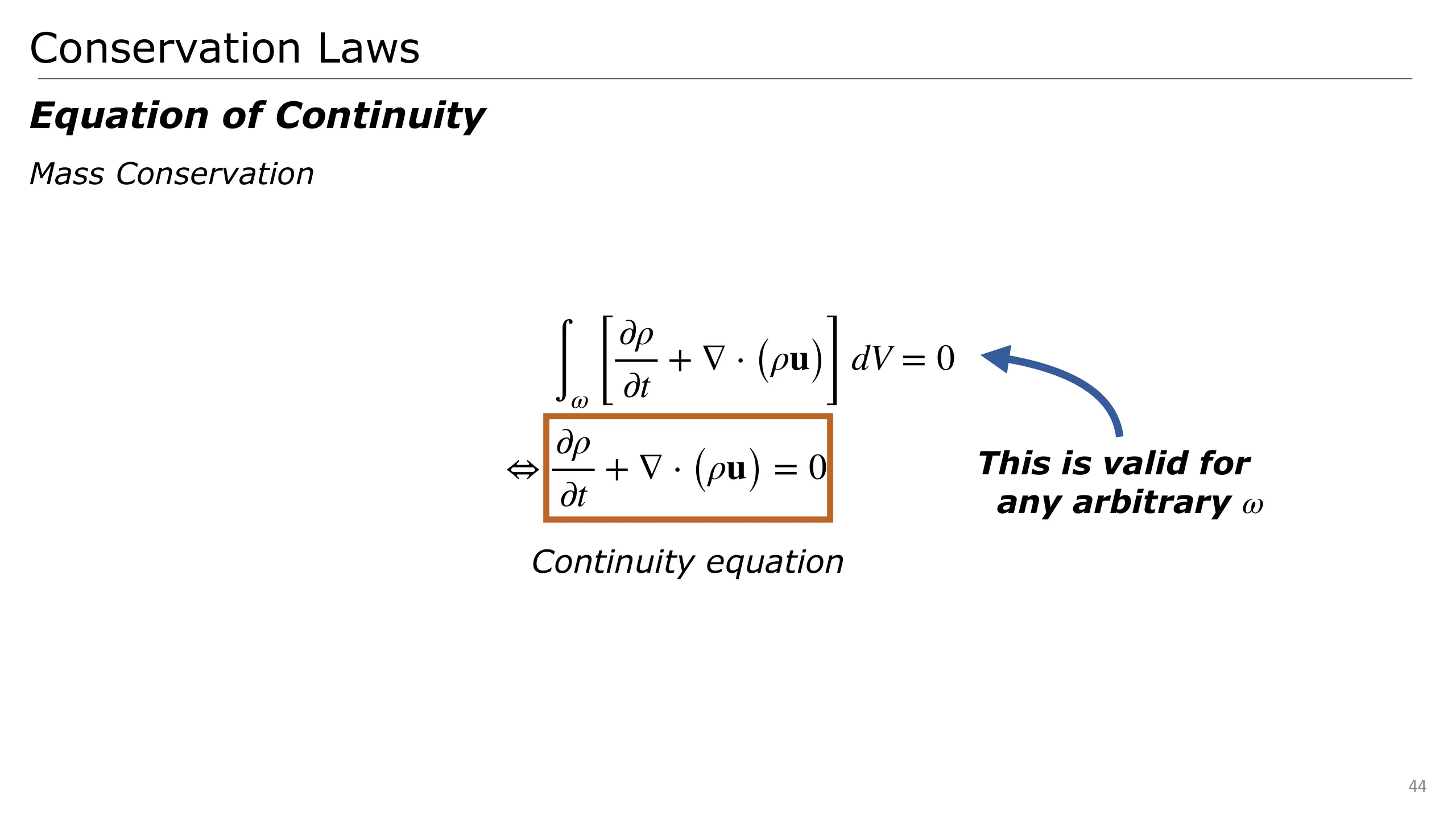
We can finally notice that since omega is arbitrary, it must be true for every omega.

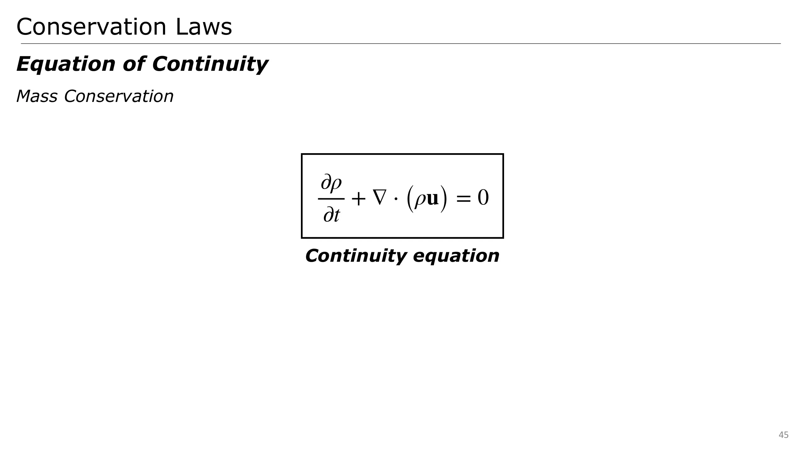
Then, we obtain the so-called continuity equation stating that the change of mass equals how mass exits and enters the system.

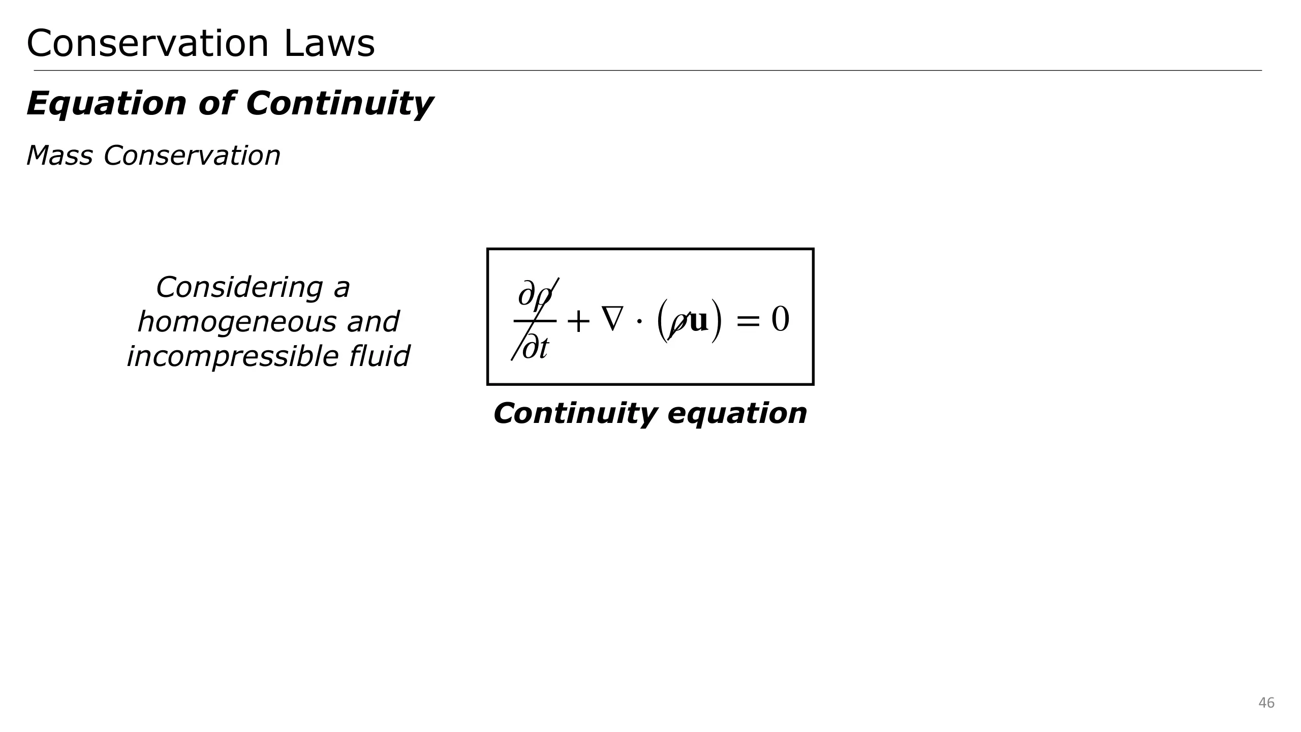
What is very important in our context is that, when a fluid is incompressible and homogeneous, density is constant in time: the fluid cannot concentrate further or become sparser at any point

Thus, density derivatives cancel in our continuity equation.

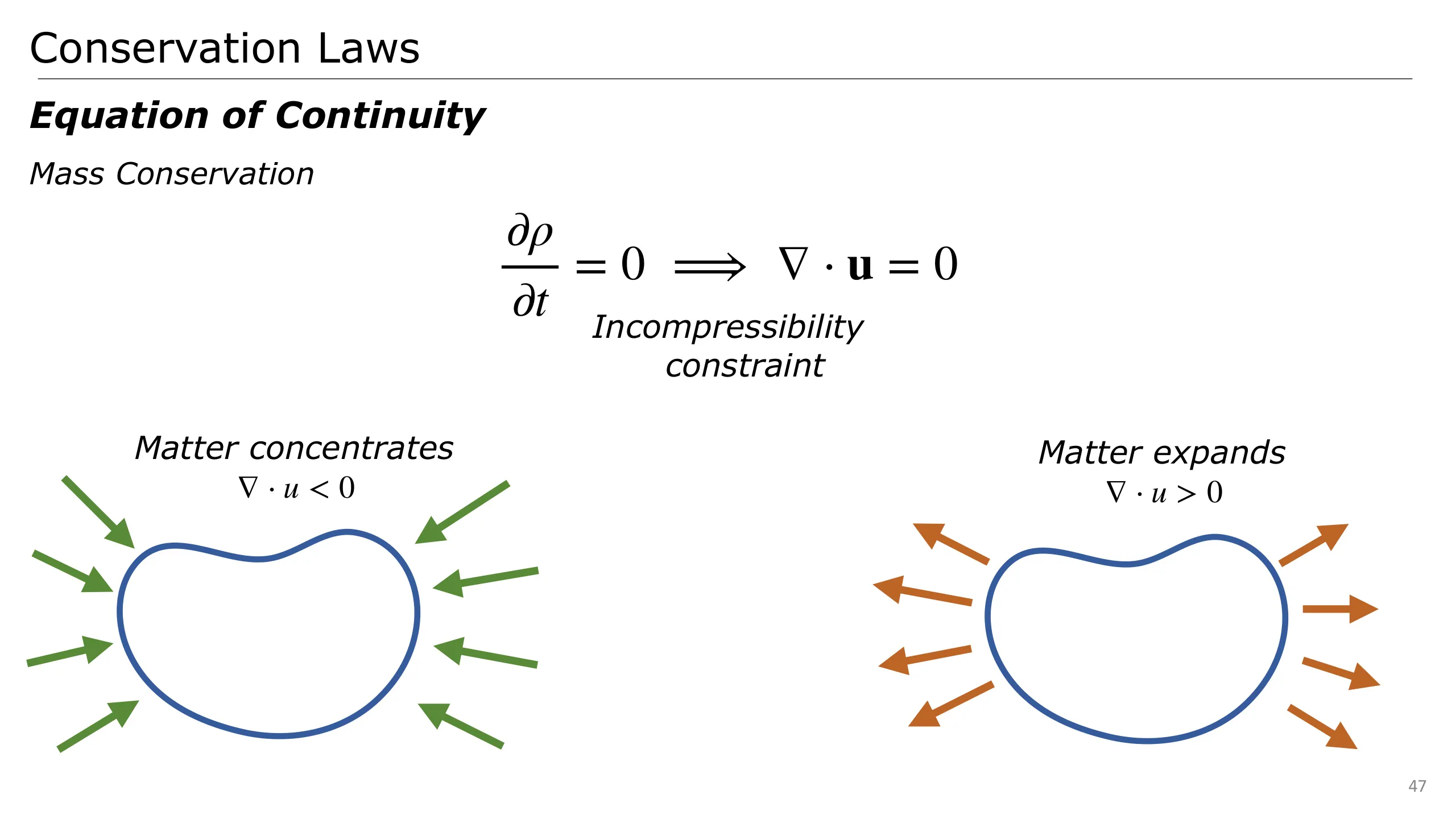
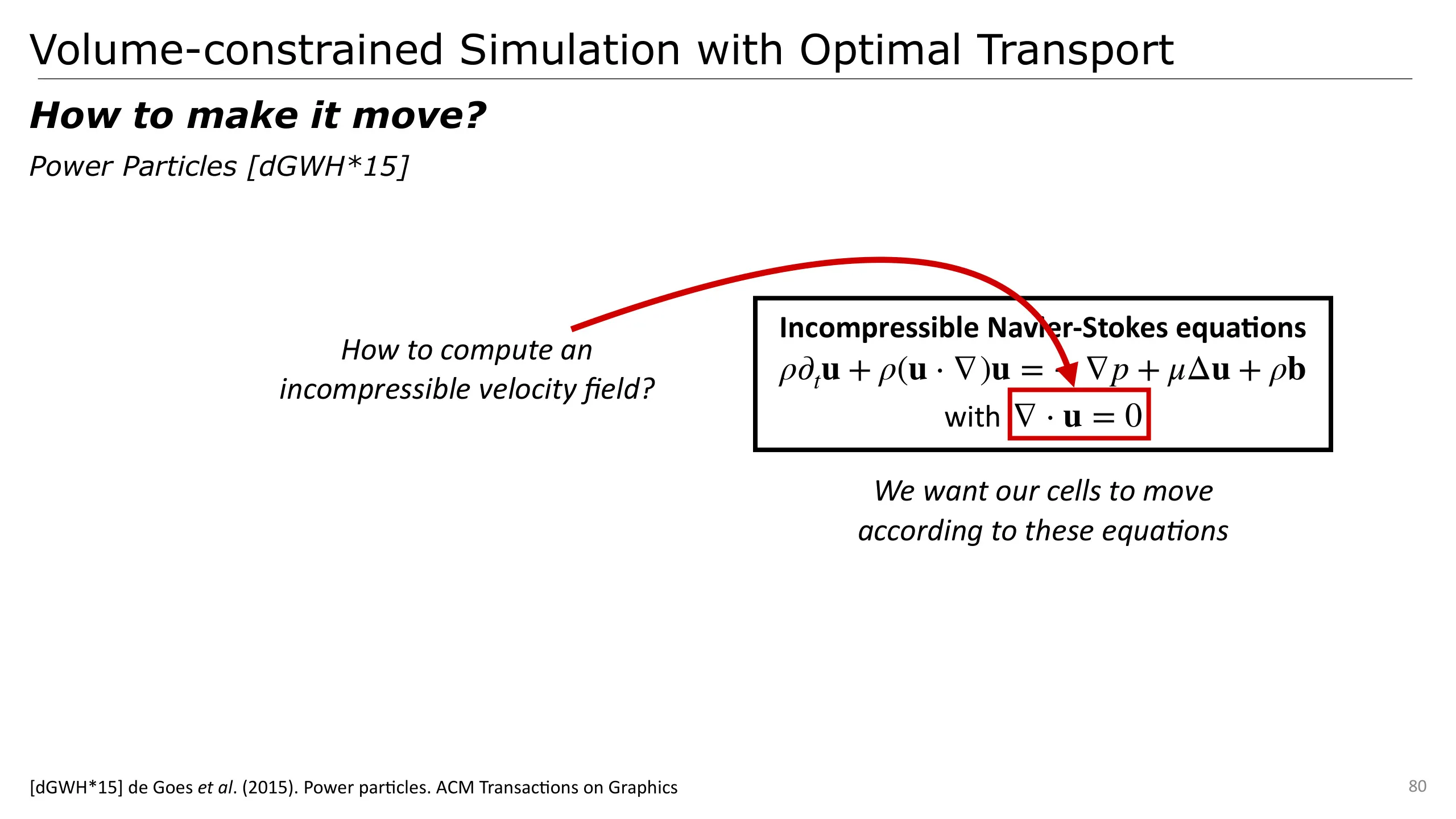
Thus we can drop the terms linked to the rate of change of density in time, and we obtain the incompressibility constraint of the velocity field.

This can be better understood from the properties of the divergence operator. As the local flux, it describes the balance between what goes in and what goes out.

In such case, it directly gives us the information on how the matter concentrates or expands.

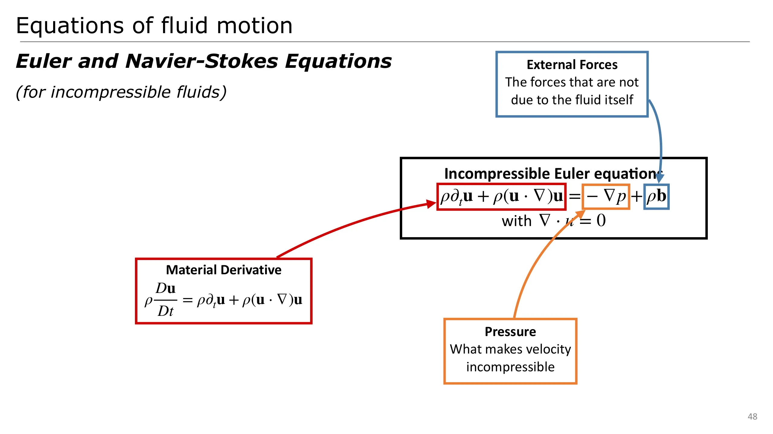
Once we know the conservation laws that dictate the motion of our fluid, we can assemble them in a set of equations called the Incompressible Euler equations.

I quickly summarise what are their components.

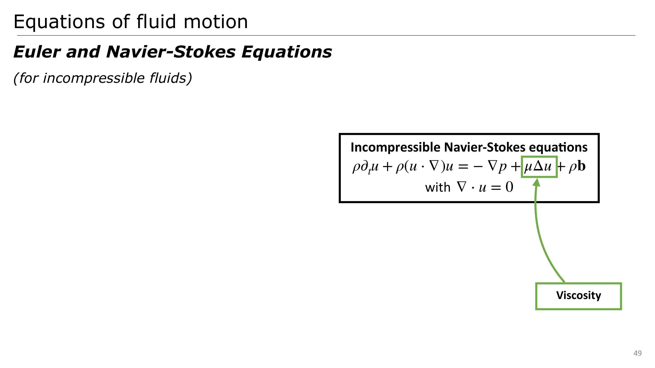
Adding the viscosity force to these equations finally results in the Navier-Stokes equations.

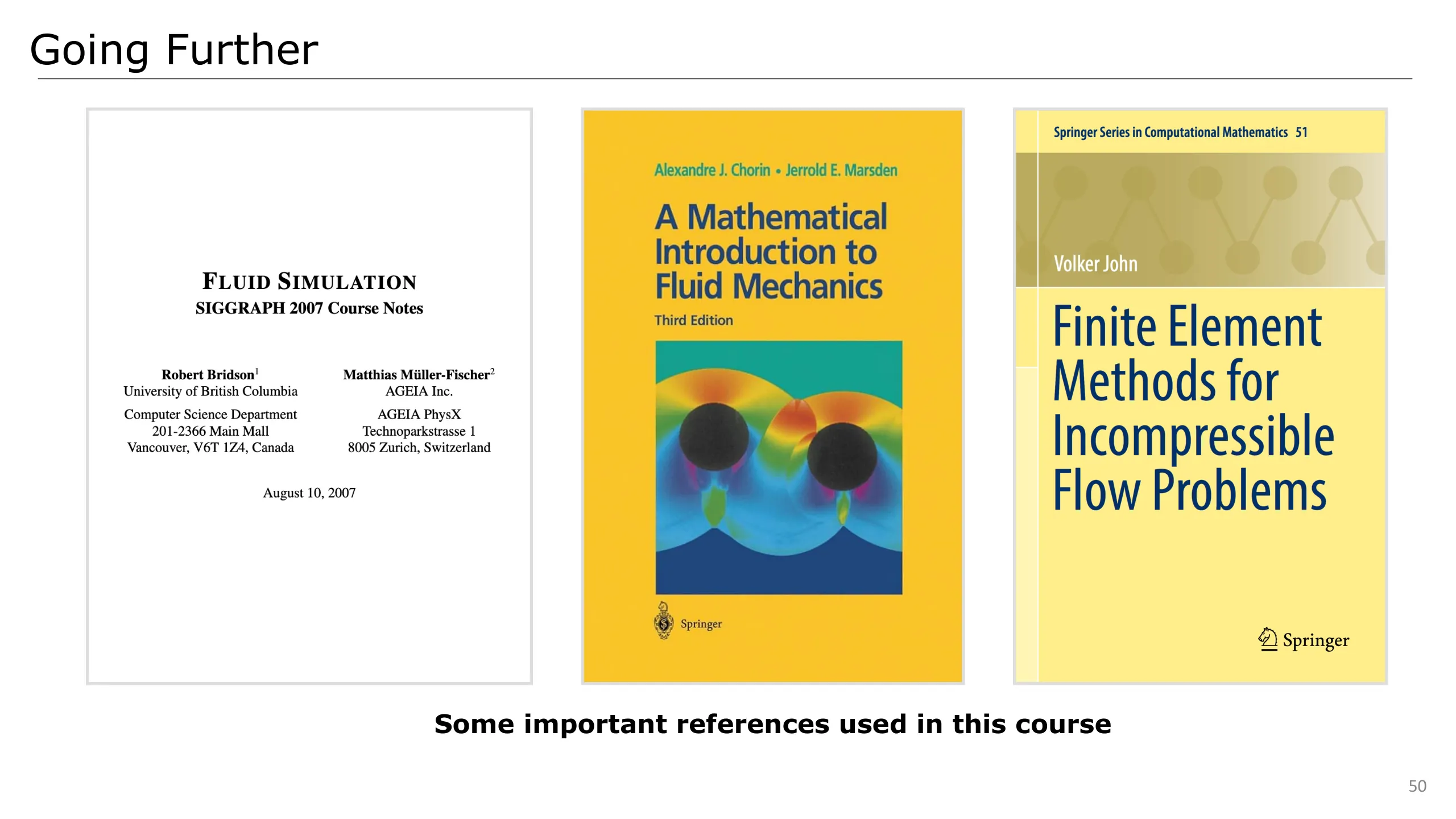
This ends the physics I wanted to describe before entering the heart of the matter.
I also wanted to mention my main references that go into more detail and rigour of what I introduced.
Those are really nice and I truly encourage you to get into those if this is something that you’re interested in.

Once we know what is the model of the physics we want to actually simulate, we have to discretise it.

This discretisation must be performed in time and in space

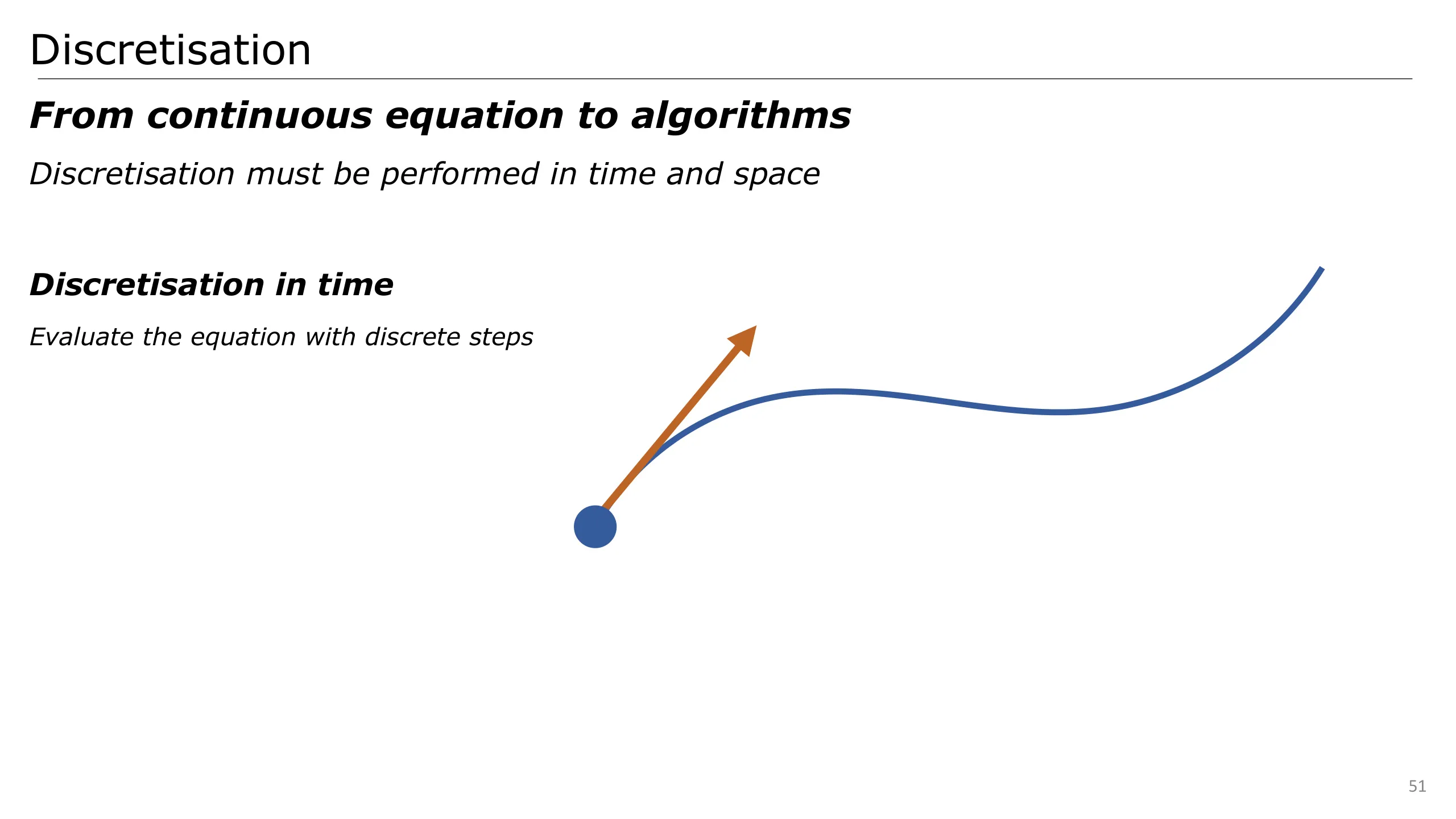
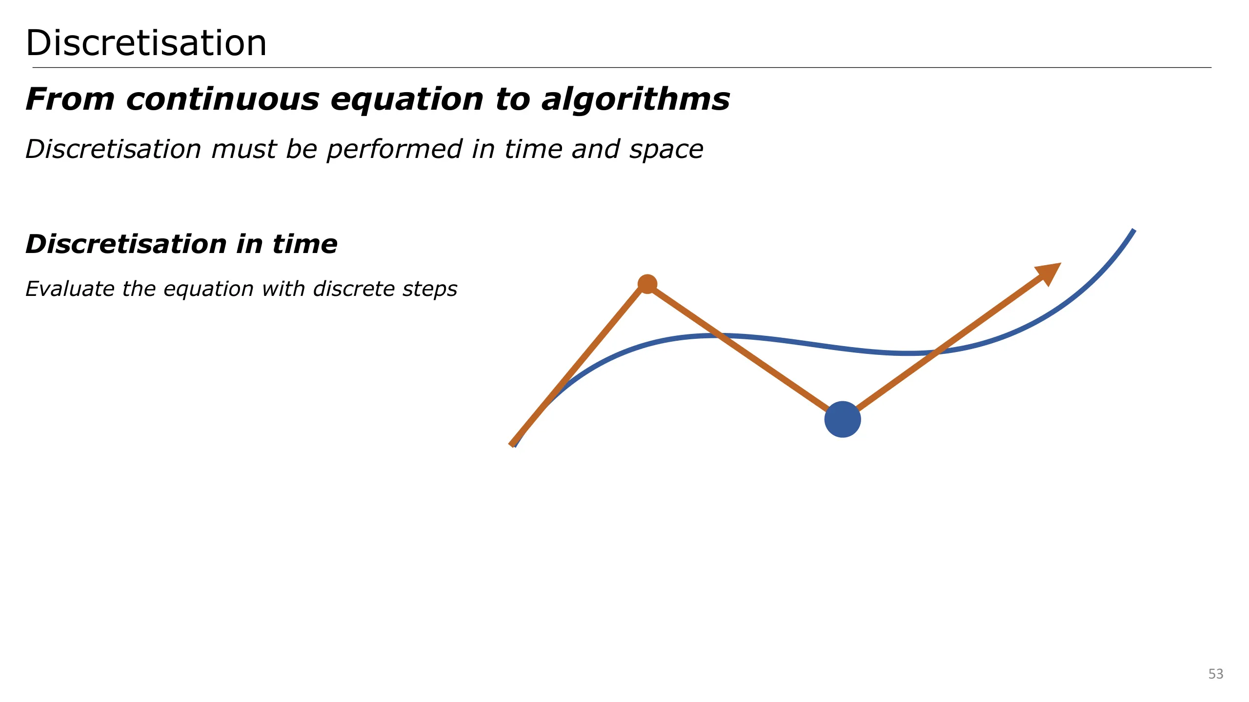
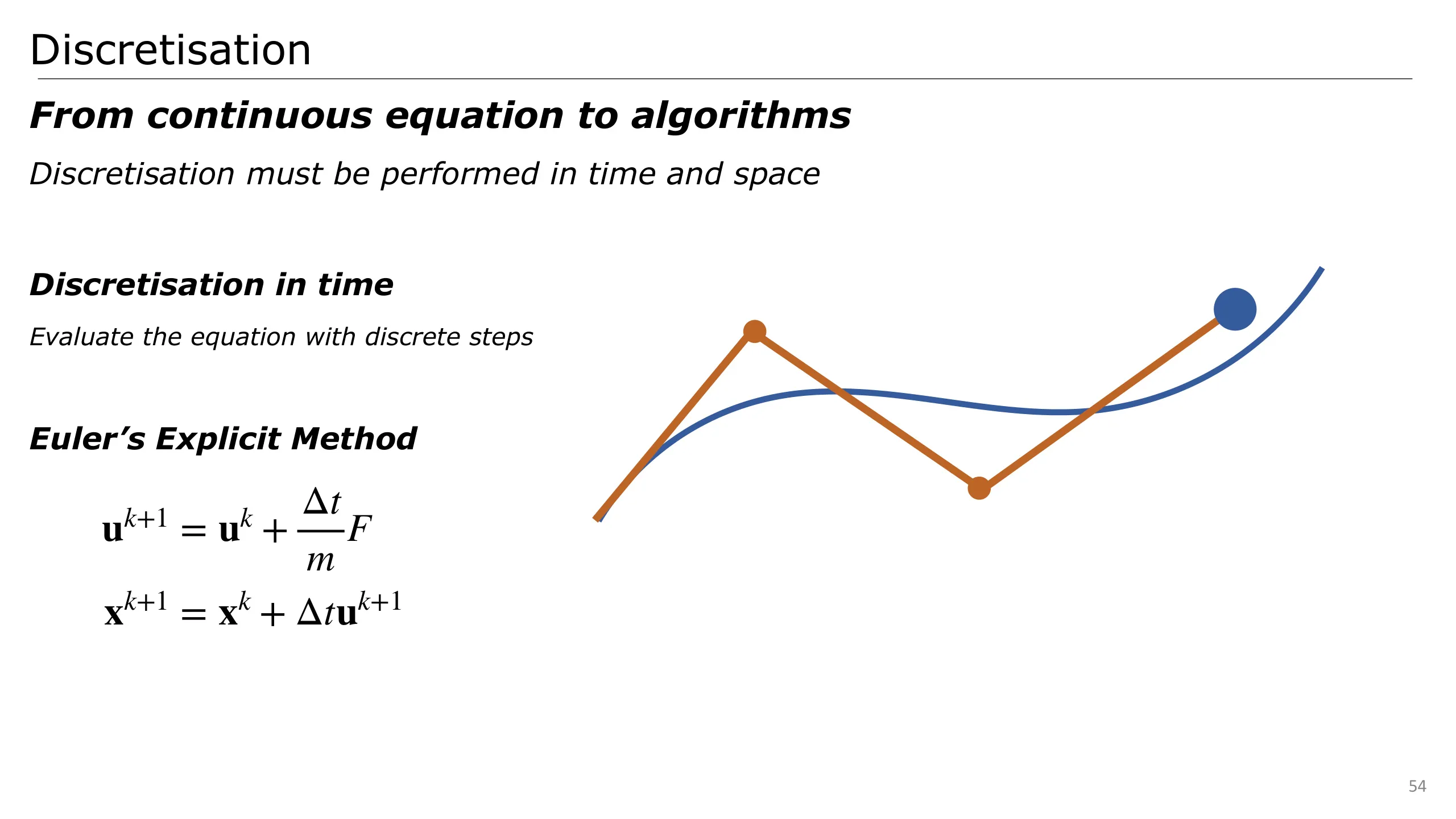
In time, this means to perform discrete steps over the function we are integrating.

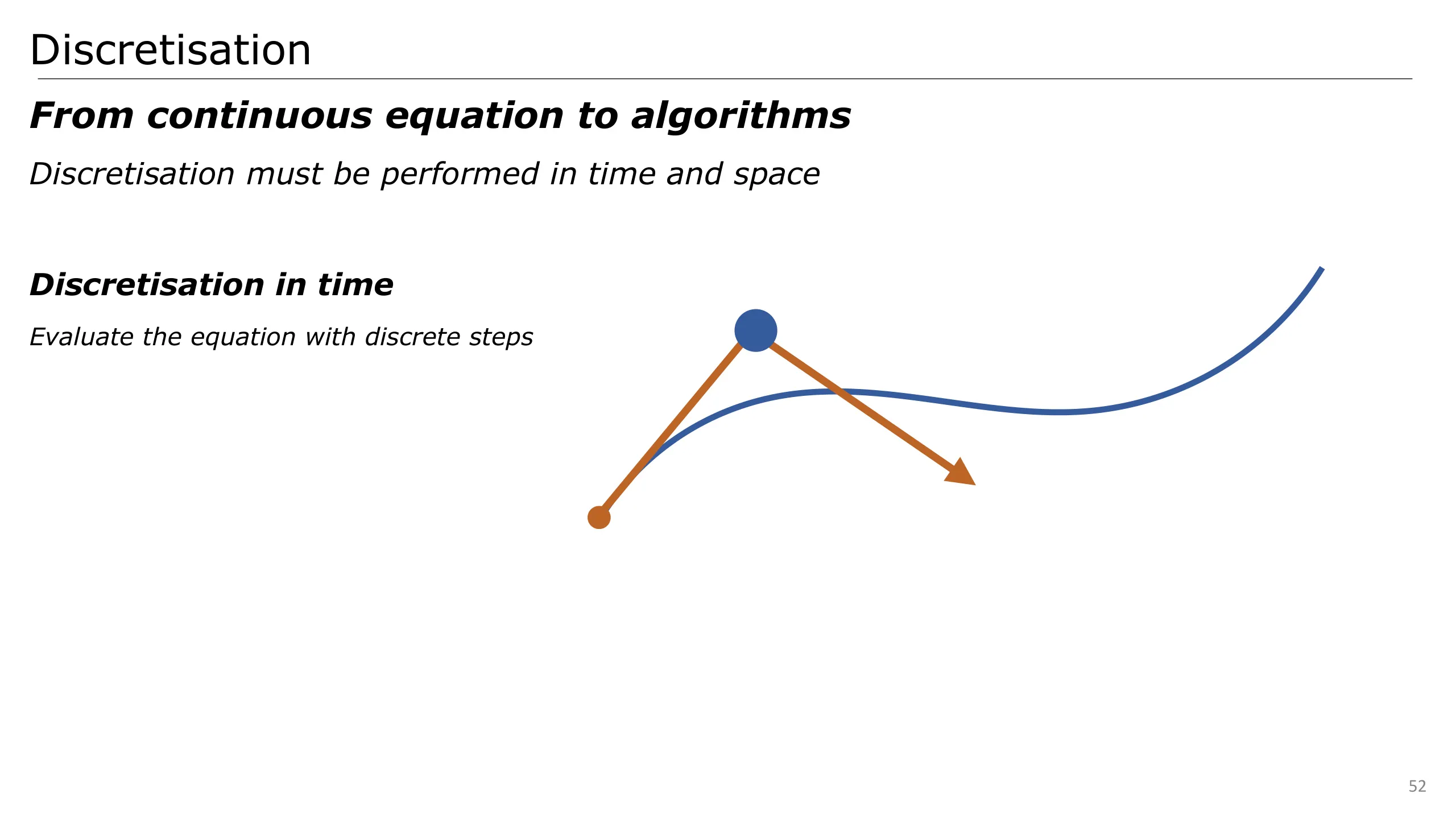
This can be done in a super simple way by just following the direction of the derivative iteratively to find the next point.

This discretisation is called Euler’s Explicit Method. We are taking fixed steps along the derivative at the current point.
To actually insert it into our simulation, we can rely on Newton’s 2nd law to compute the next velocity, and use this value to update the position.

Note that this is a very simple approximation and has many drawbacks related to the fixed parameter size.

Other discretisations are more robust and can be considered if required.

Then we have to actually discretise our function in space.

This leads to two main questions: where to position the samples and how do their values and positions change in time?

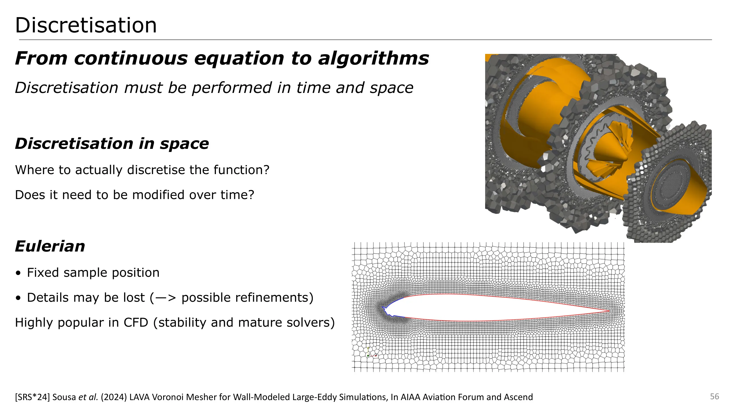
One main class of method uses an Eulerian point of view through a fixed grid.

This is a very popular method in CFD since it enables various very robust and stable solvers.

Since the grid is fixed, it can lead to aliasing if it is too coarse where we actually want details.

The simulation domain must then be discretised adaptively or during the simulation.

This strategy is commonly implemented in CFD for the discretization of Navier-Stokes equations for their accuracy but requires a lot of computation power.

A very popular alternative is the Lattice Boltzmann Method (LBM).

In contrast with methods targeting the discretization of Navier-Stokes equations describing a macroscopic field, LBM targets Boltzmann equation describing a mesoscopic field

This method received a growing interest in CFD and graphics since the algorithm is quite simple and can be parallelised very efficiently.

It enables large scale simulations producing very impressive effects.

Another point of view is using moving particles that follow the matter in a Lagrangian way.

This is nice since it provides details where needed in the simulation which is very much appreciated in graphics.

Multiple particle-based methods have been proposed by relying on either:

- a mesh which provides precision but needs update to avoid tangling

- particles only (or mesh-free) but can require elaborate schemes to estimate differentials or enforce volume conservation

One last line of work is represented by the hybrid methods.

Those are hybrid in the sense that they combine a Lagrangian and an Eulerian POV to benefit from their respective strengths

While particles accurately and efficiently follow the matter, they can lead to inaccurate estimation of differentials or surface quantities in case of mesh-less representation.

On the other side, a grid provides a very accurate estimation of the forces but can lead to aliasing and loss of details

To benefit from both these strengths, hybrid methods rely on particles to follow the matter and on a grid to compute the forces.

This allows a very wide range of effects: granular materials, or incompressible fluids

Once that we know those characteristics, we can try to develop a new POV to benefit from the advantages of these representations.

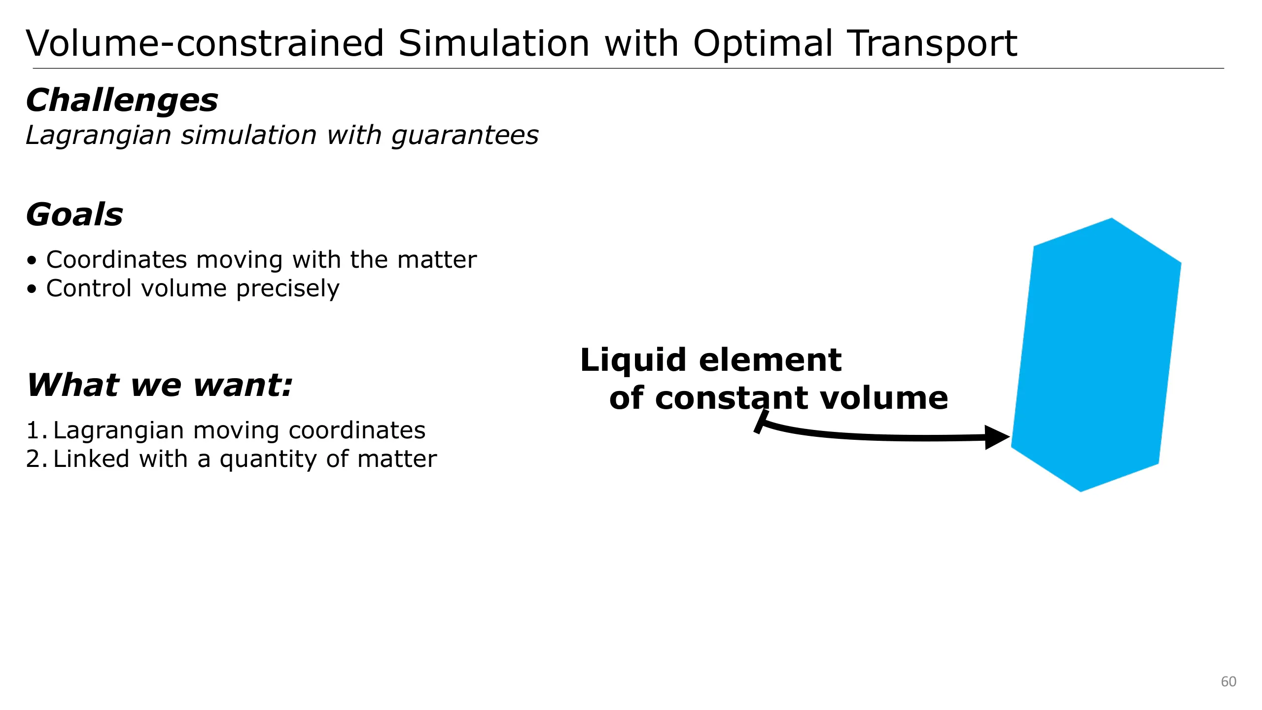
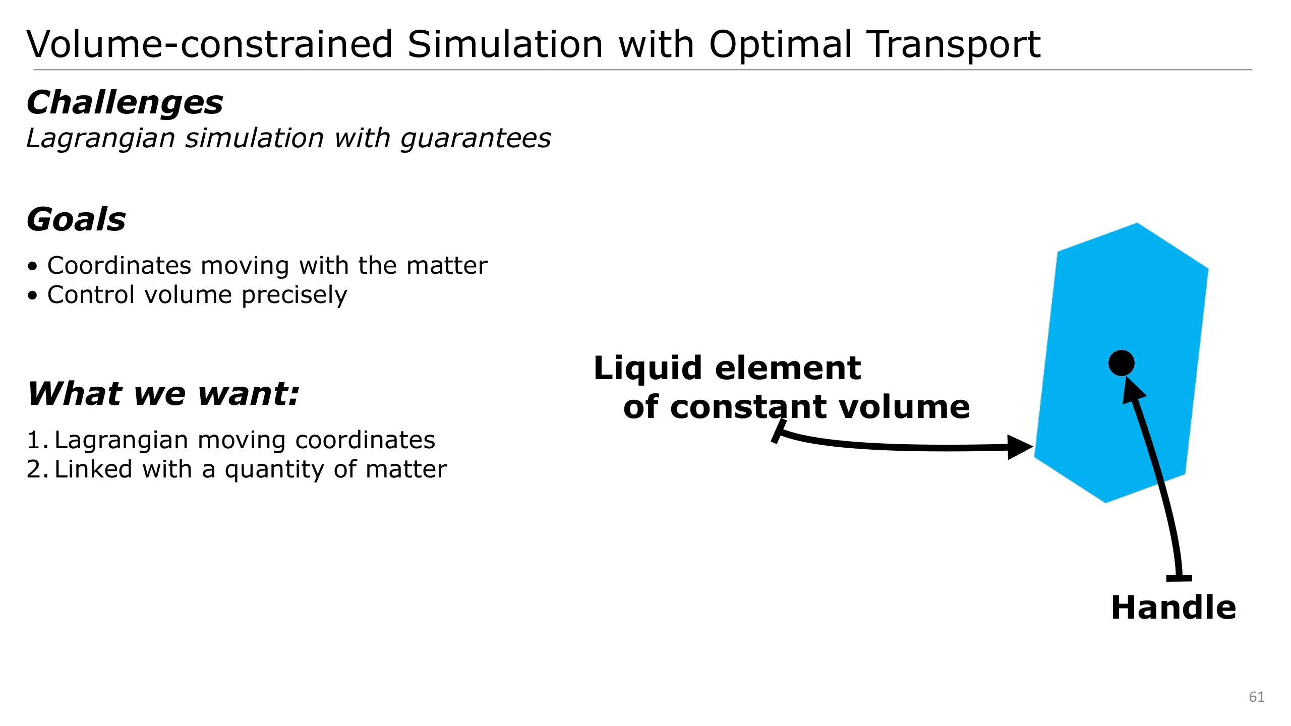
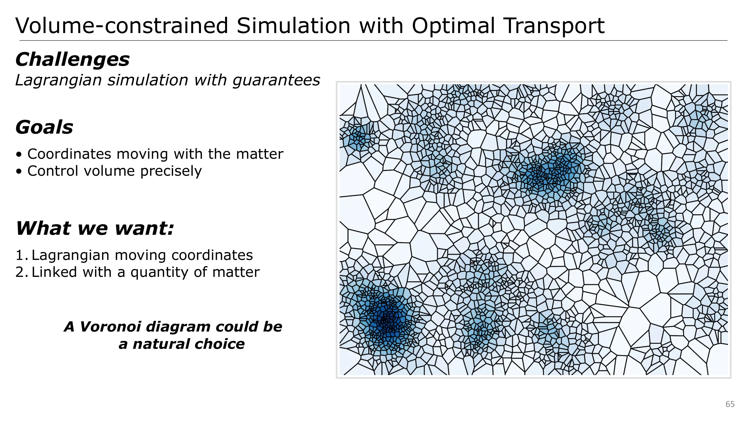
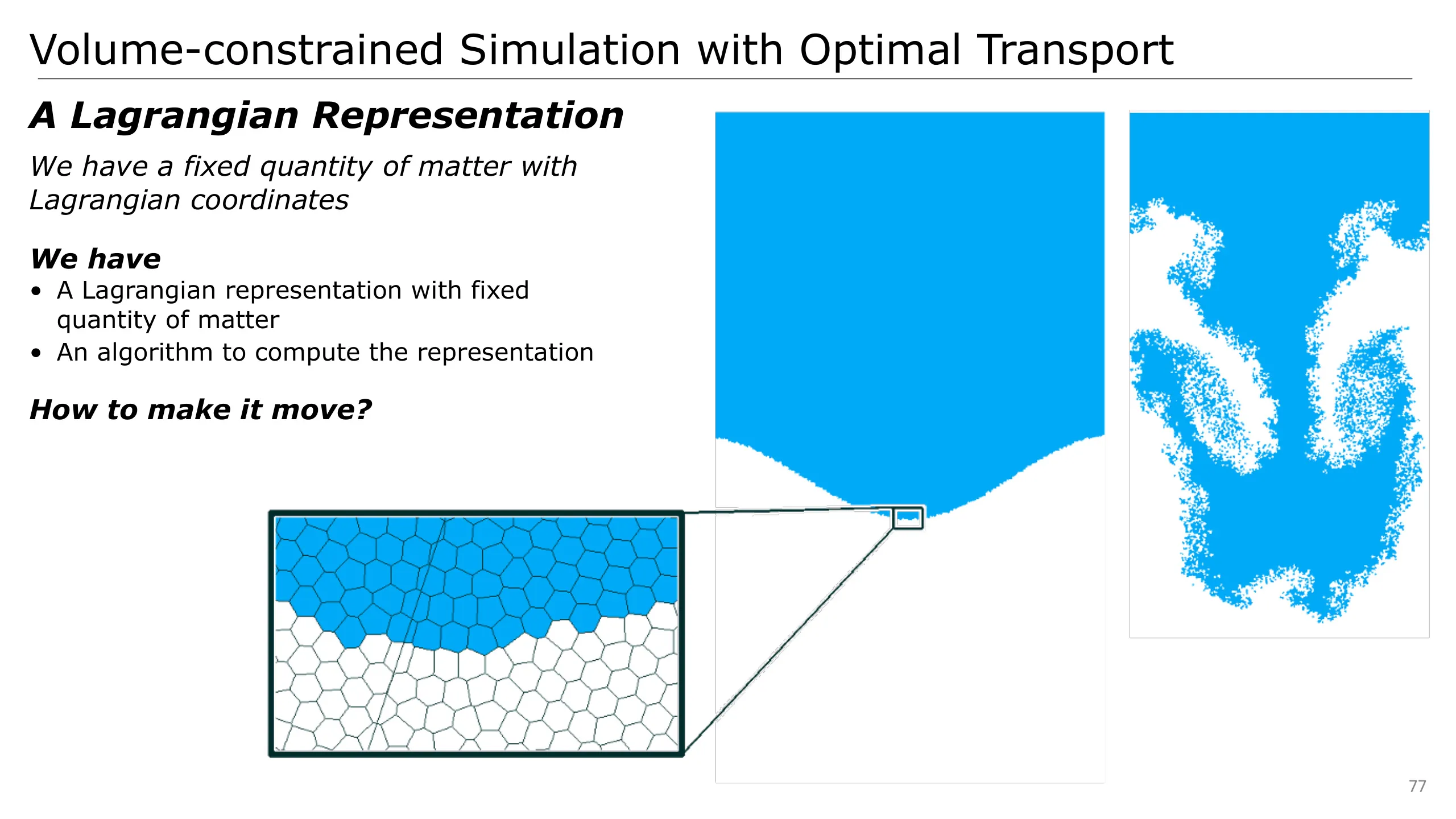
We want coordinates moving with the matter in a Lagrangian way to benefit from its advantages.

But in the same way, we want to control precisely the volume of fluid they are holding by design.

For that, we can consider a set of moving coordinates…

And link each of them with a quantity of matter

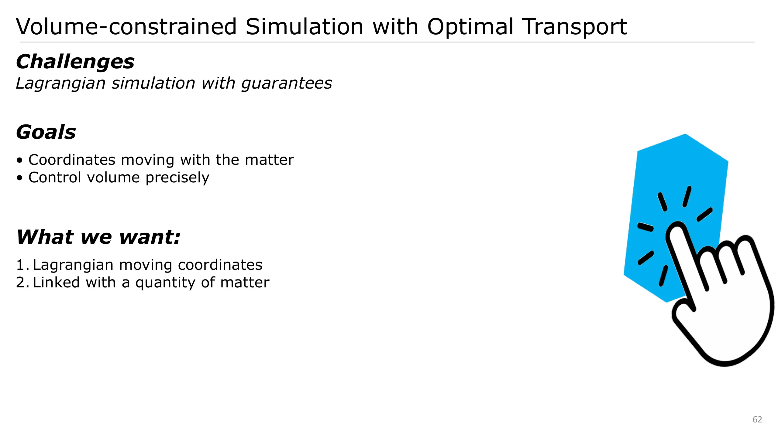
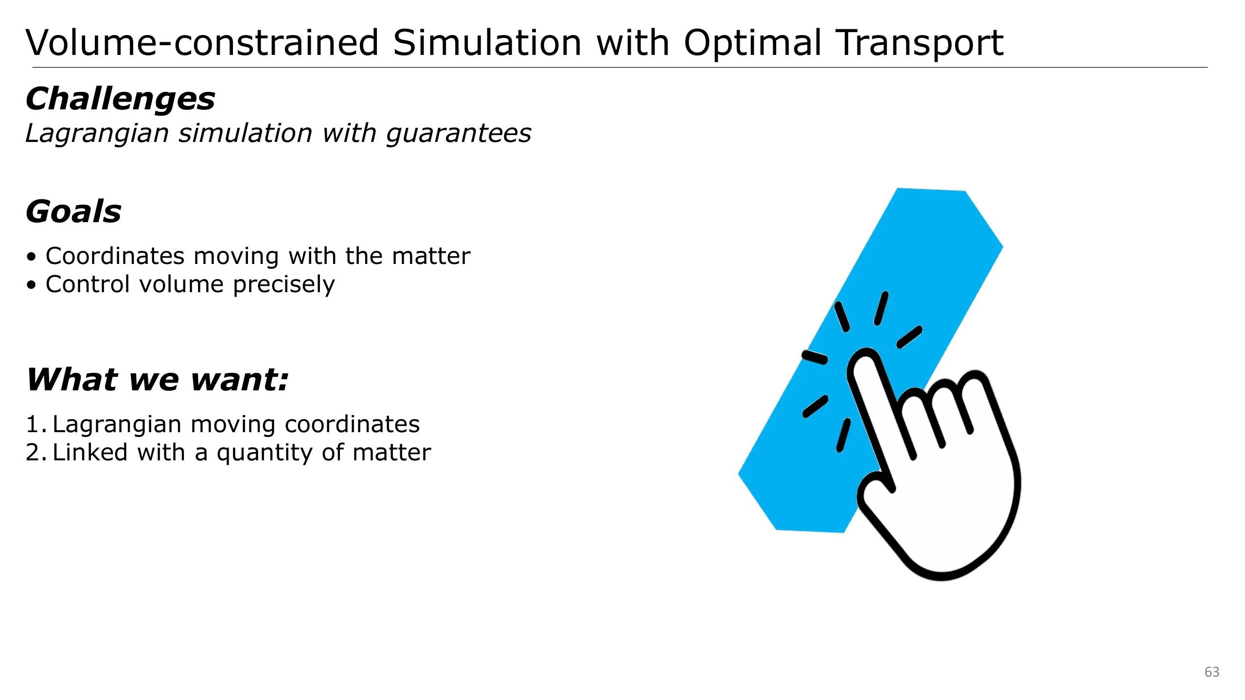
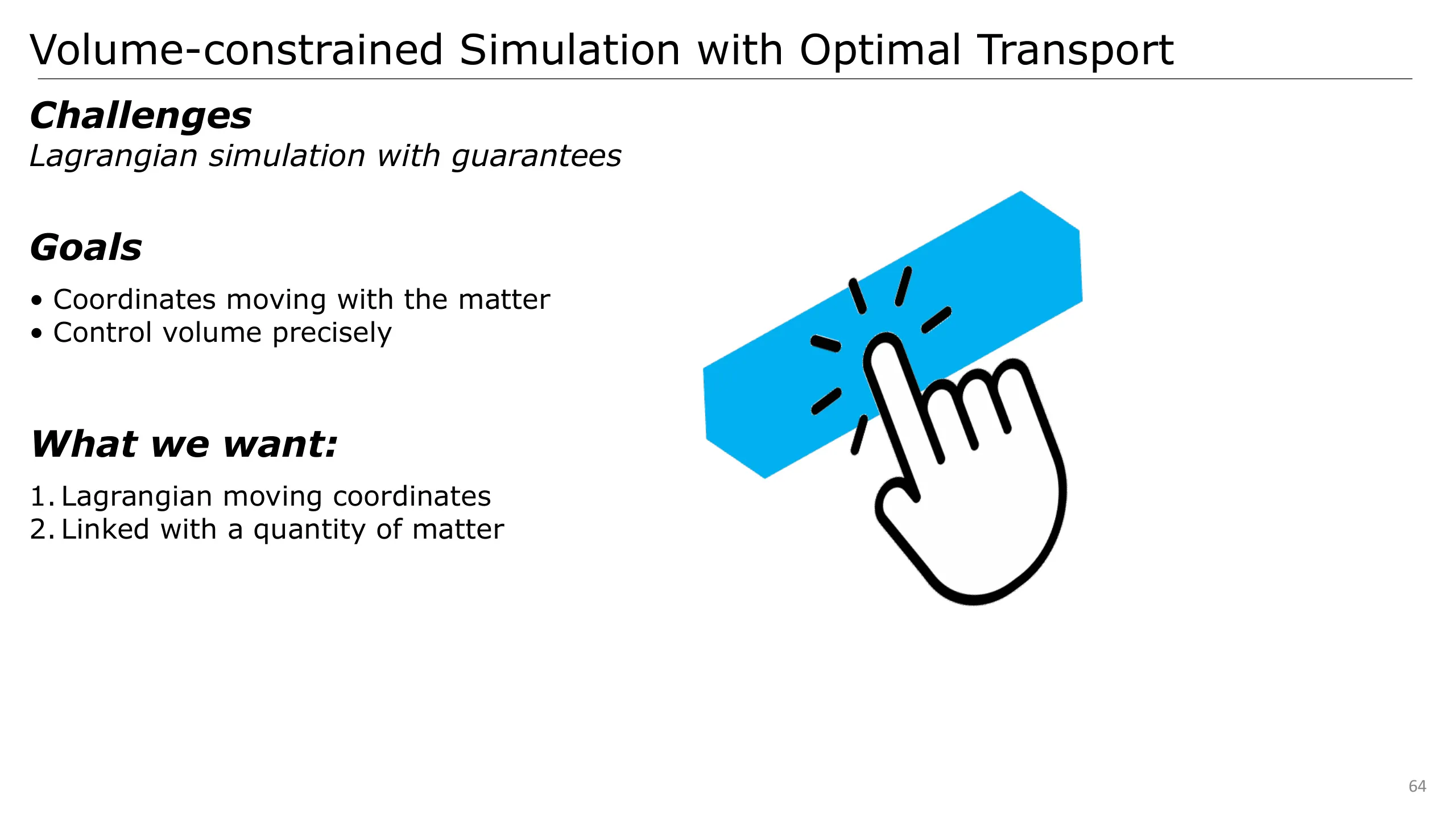
We also want to be able to move this liquid element, through a kind of handle.

With these constraints, a Voronoi diagram seems like an interesting choice.

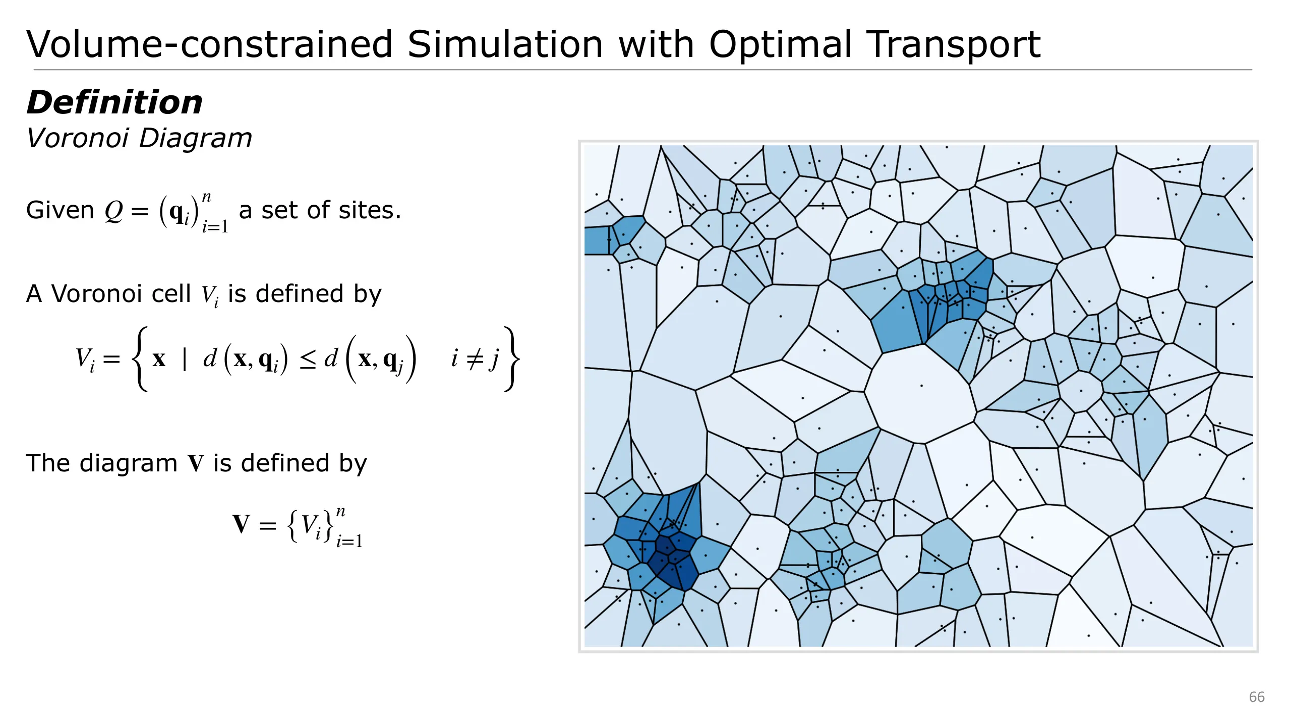
We first take a closer look at this structure.

A Voronoi diagram is parametrised by a set of sites, here some points in 2D drawn in black.

Each site is linked to a cell of the Voronoi diagram which is composed of all points closer to the site of the current cell than any other site.

The diagram is then finally given by the set of all cells.

Note: a bisector is composed of every point at equal distance of two sites. Those are facets when considering a given cell.

A vertex of a cell is a vertex of the polytope bounding the cell.

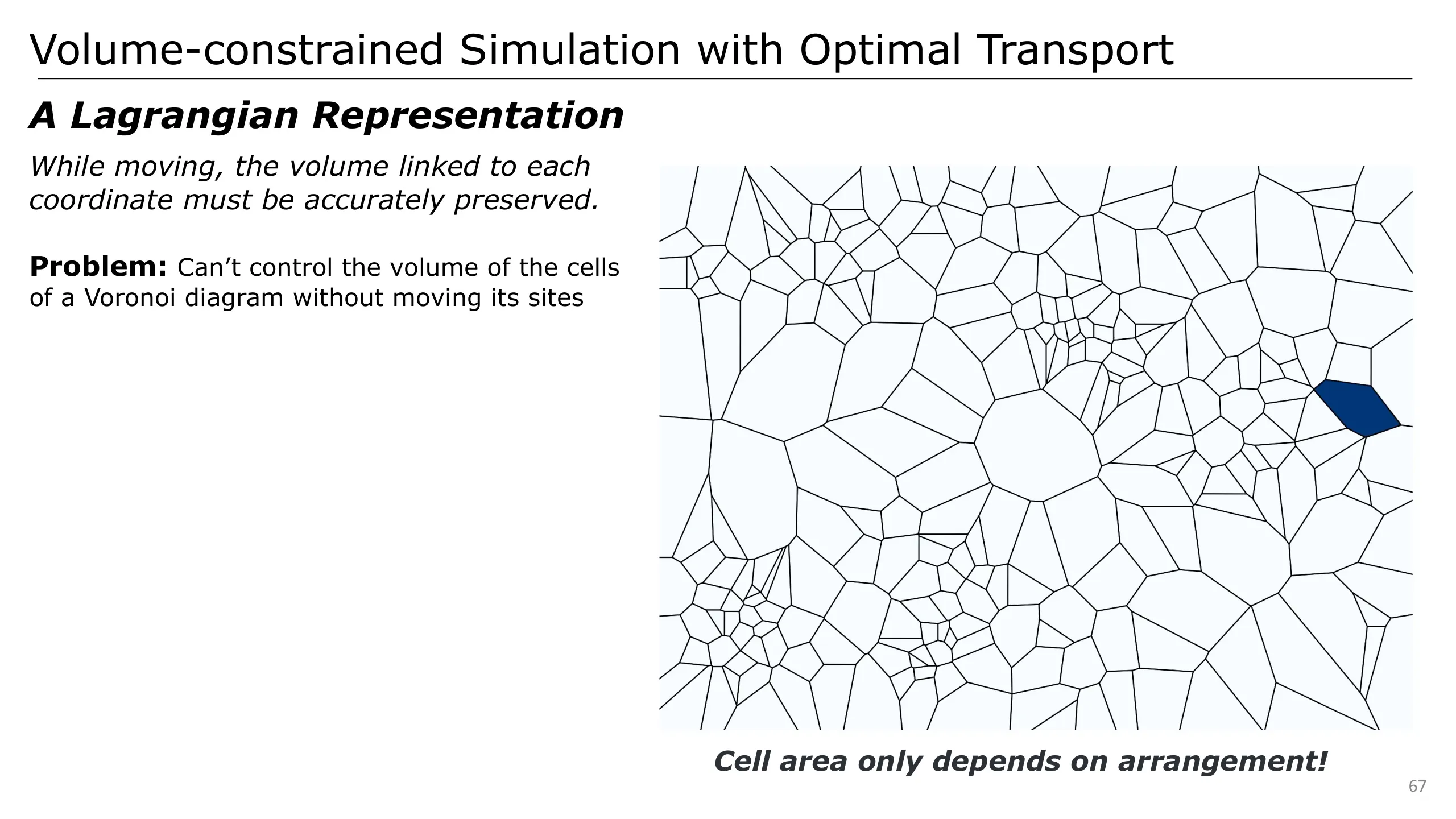
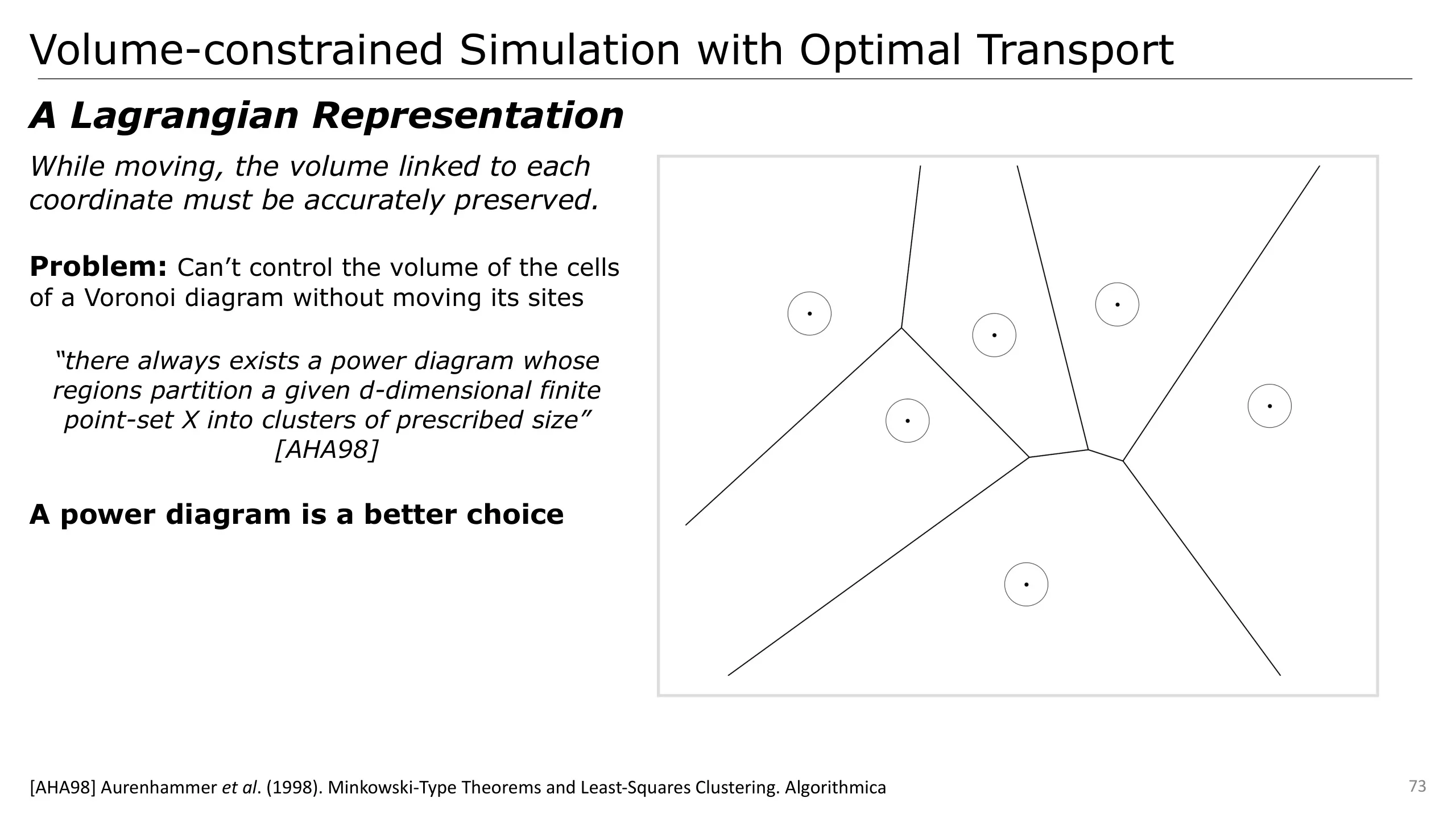
Coming back to our fluid modelling, the problem is that we cannot guarantee that the volume of each cell of a Voronoi diagram does not change over time.

As we can see on the right, if I’m moving the site of a cell (in blue), its volume clearly changes.

Worse, we have no other way than changing the position of the site to modify its area.

We then need an additional degree of freedom to address this issue.

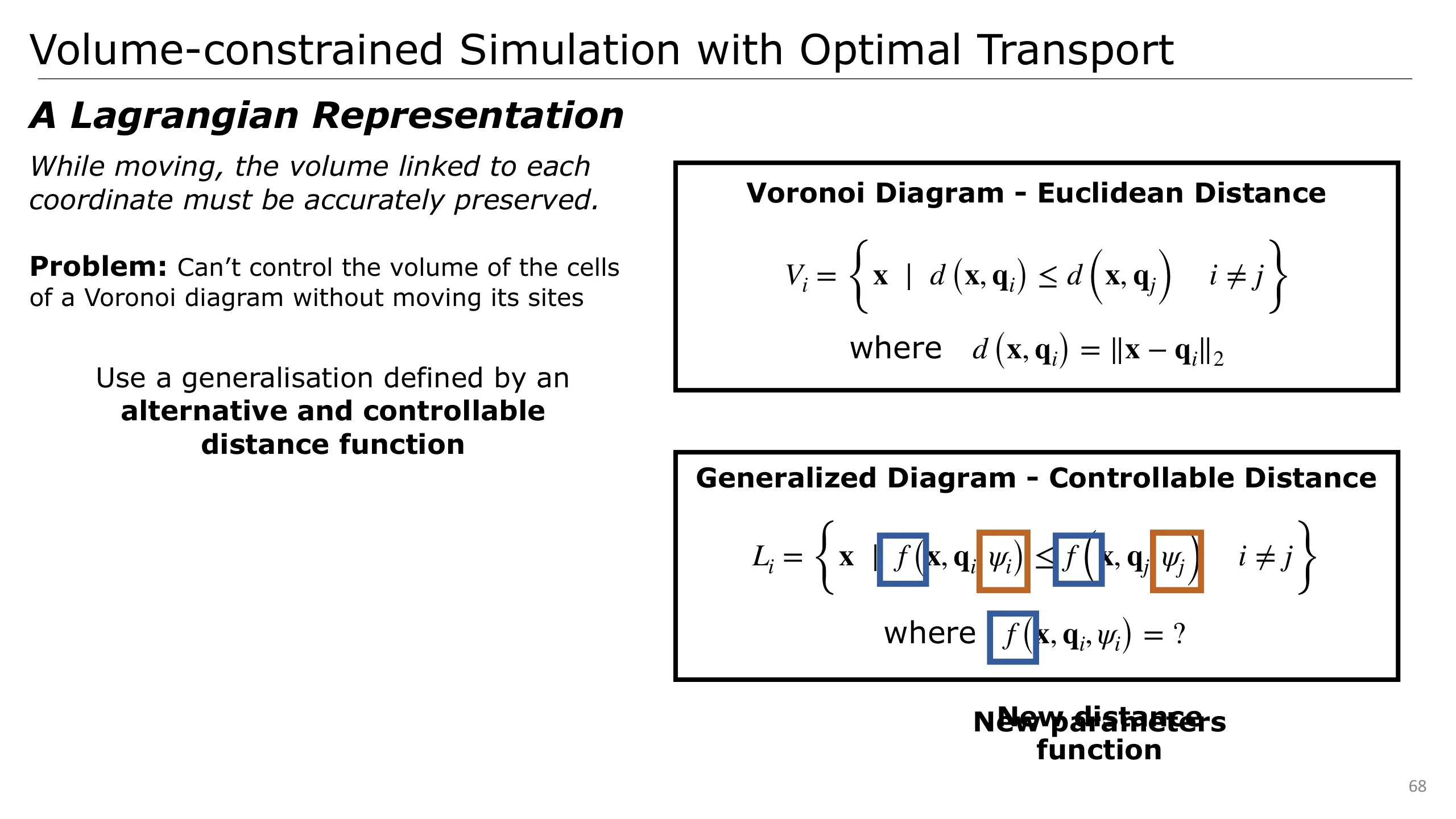
For that, let’s first consider Voronoi diagrams. Each cell of a Voronoi diagram is characterised by all points closer to the site of the cell than any other site.

For a Voronoi diagram, “closer” is evaluated from the Euclidean distance.

We can change this distance for another one like in the bottom, which takes into account an additional degree of freedom, here psi.

So we have this new degree of freedom psi, which is a parameter that we can select

And a new distance function f that takes into account this parameter.

We now have to select this distance function.

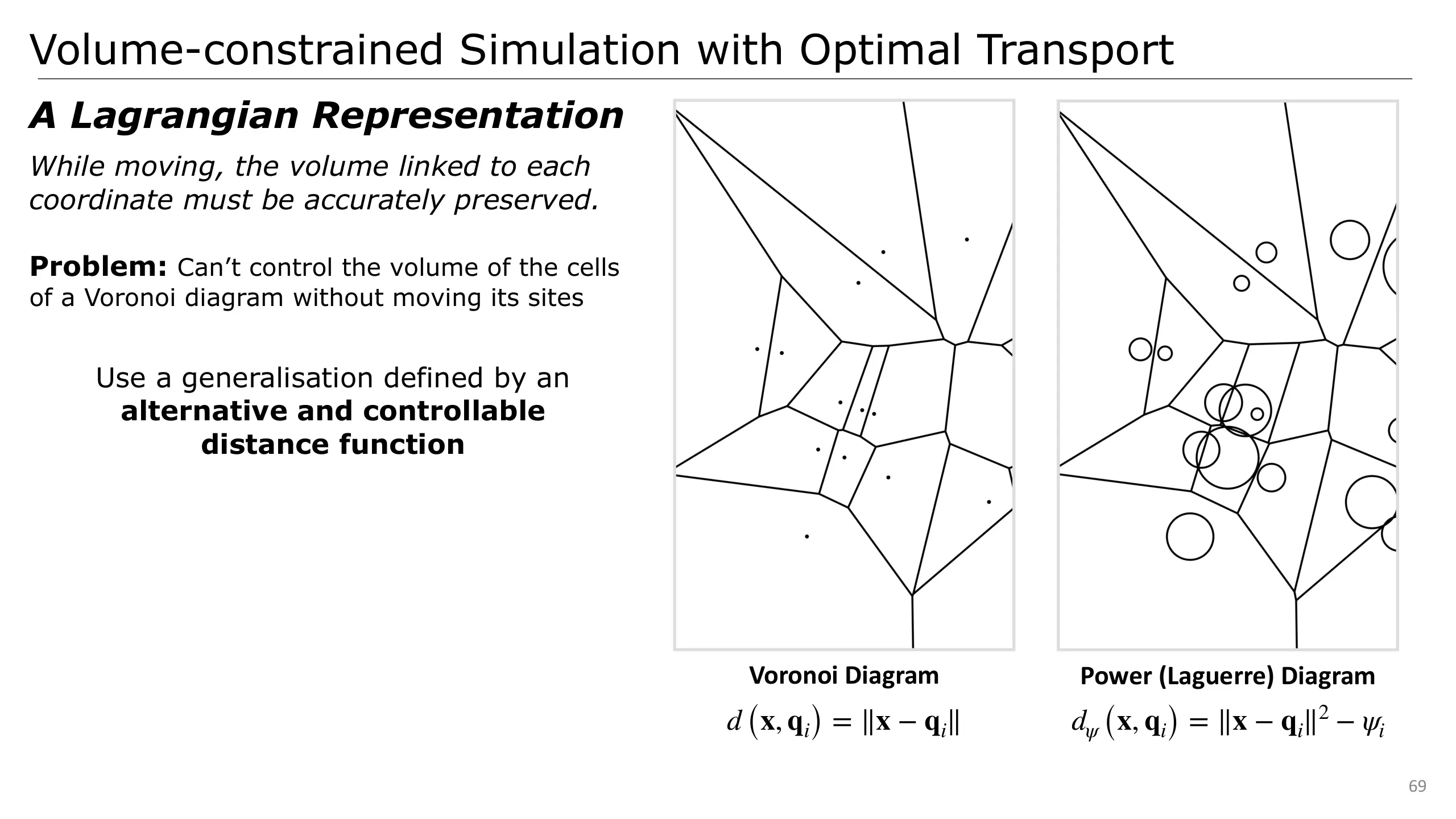
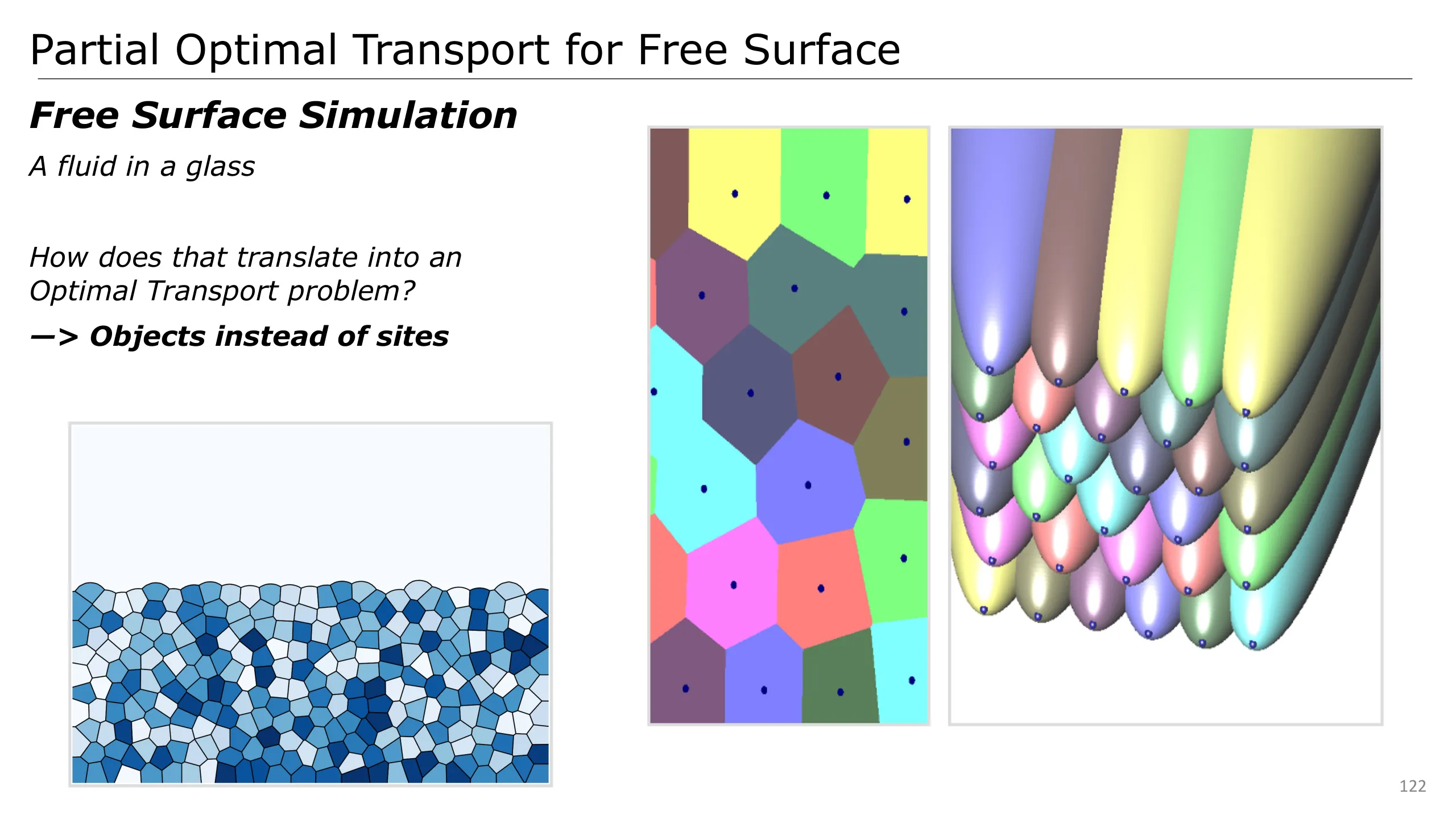
Laguerre or Power diagram offer a very interesting additional degree of freedom.

In contrast with Voronoi diagrams, these power diagrams are parametrised by a set of sites and set of scalars here named psi.

They are characterised by the Power Distance, which is the squared Euclidean distance, minus our new argument psi.

This can be interpreted as the power of a point with respect to the sphere, this is why I’m representing the sites as spheres on the schema.

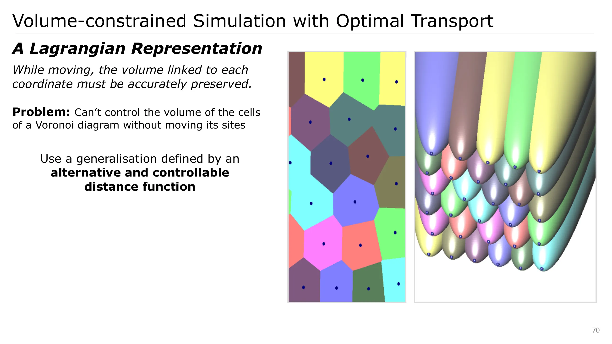
Another interpretation can be found by considering the Power diagram as the projection of a collection of paraboloids which are just the graphs of our distance functions from each site.

We can see that these graphs yield the Power diagram when seen from above.

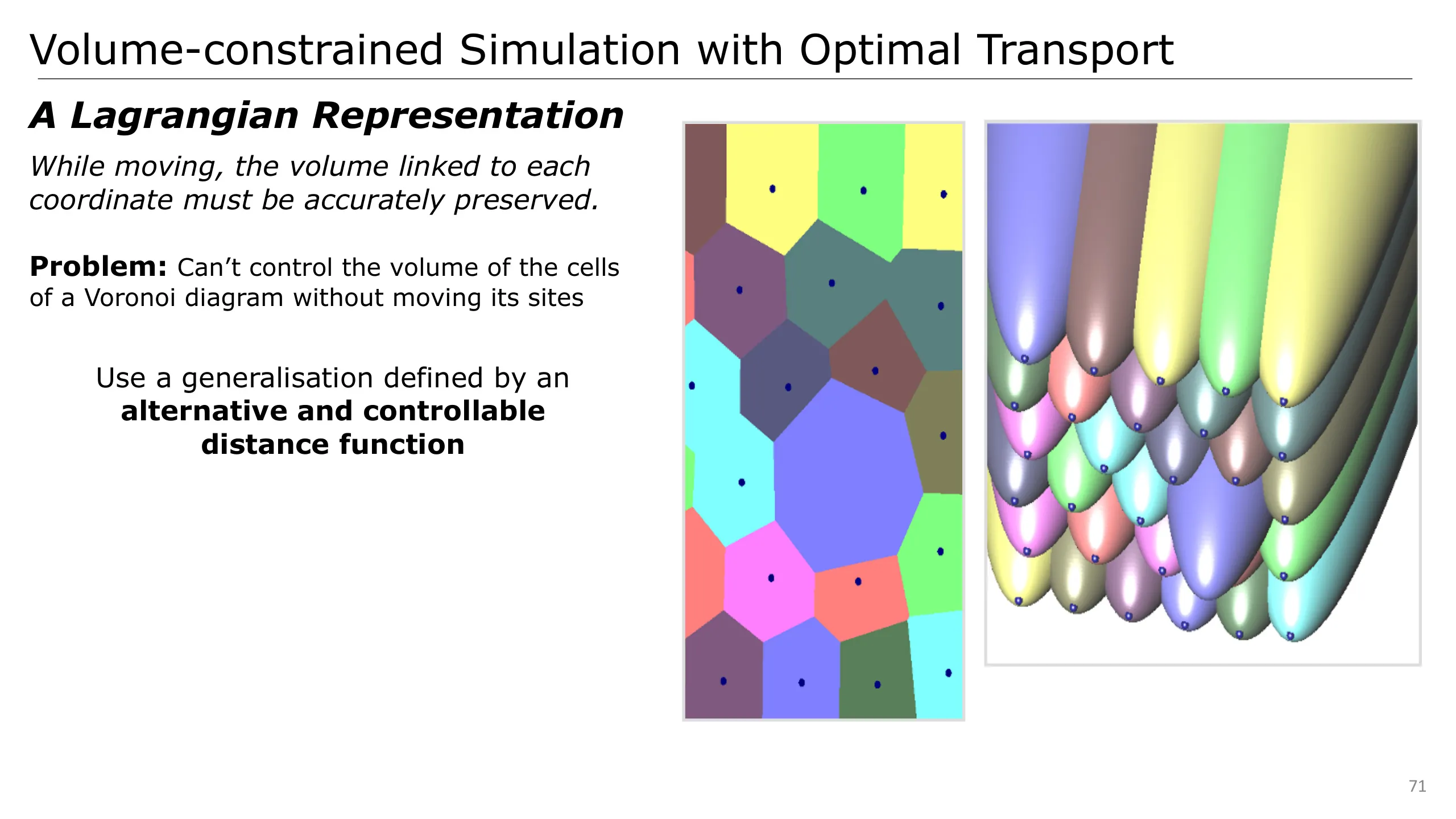
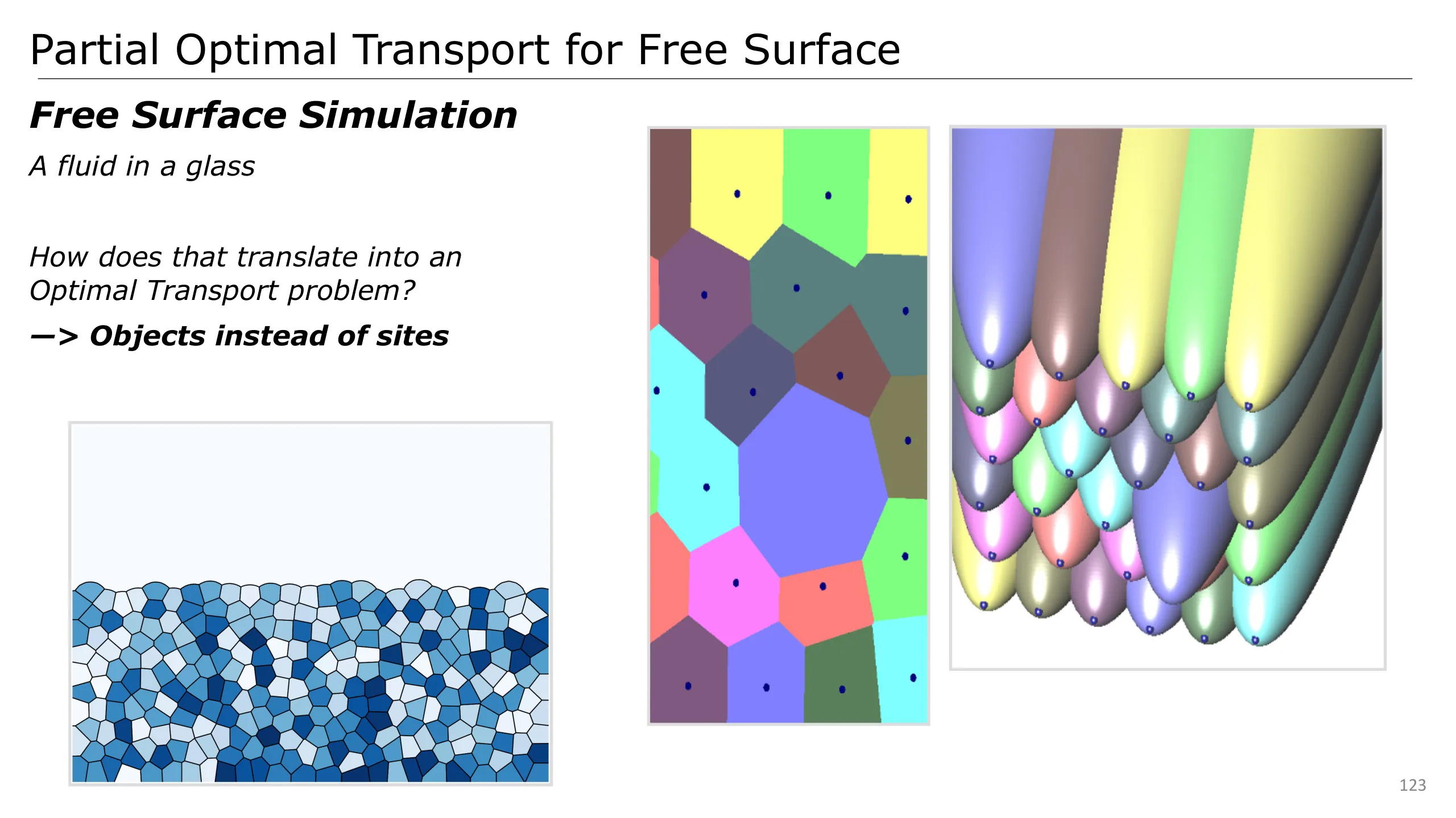
If I’m increasing our parameter psi for one of these functions, we see that it goes down, and thus, the size of the cell increases.

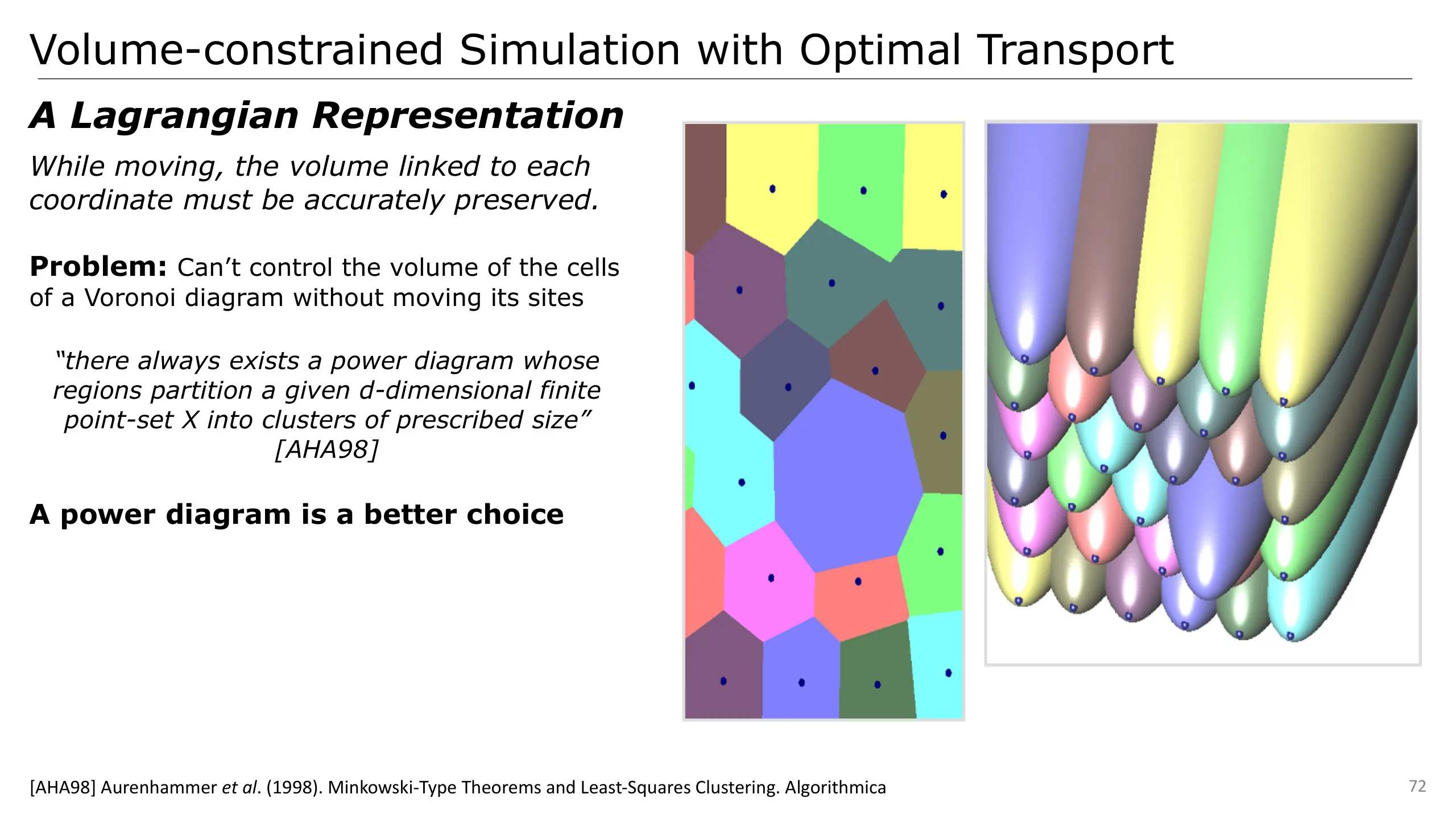
There it is, we have a way to control the volume of our cells!!

In particular, Aurenhammer et al. proved that, given a set of sites in space and a set of volumes for each of these sites, we can always find a Power diagram whose cells satisfy the given volume constraint.

This addresses our problem! We will then rely on a power diagram.

However, I must emphasise that using this new diagram, we obtain the possibility to control the volume of the cell but we also lose some characteristics of Voronoi diagrams.

Notably, the site may be located outside of its cell.

On this video, I’m increasing the parameter of the site on the left, and we can see that its cell size is increasing.

At the start of the video, sites have the same argument psi, thus the Laguerre diagram is equal to the Voronoi diagram.

If we now take a look at its bottom neighbour, we can see that while growing, it has pushed its neighbouring cell which now does not contain anymore its site.

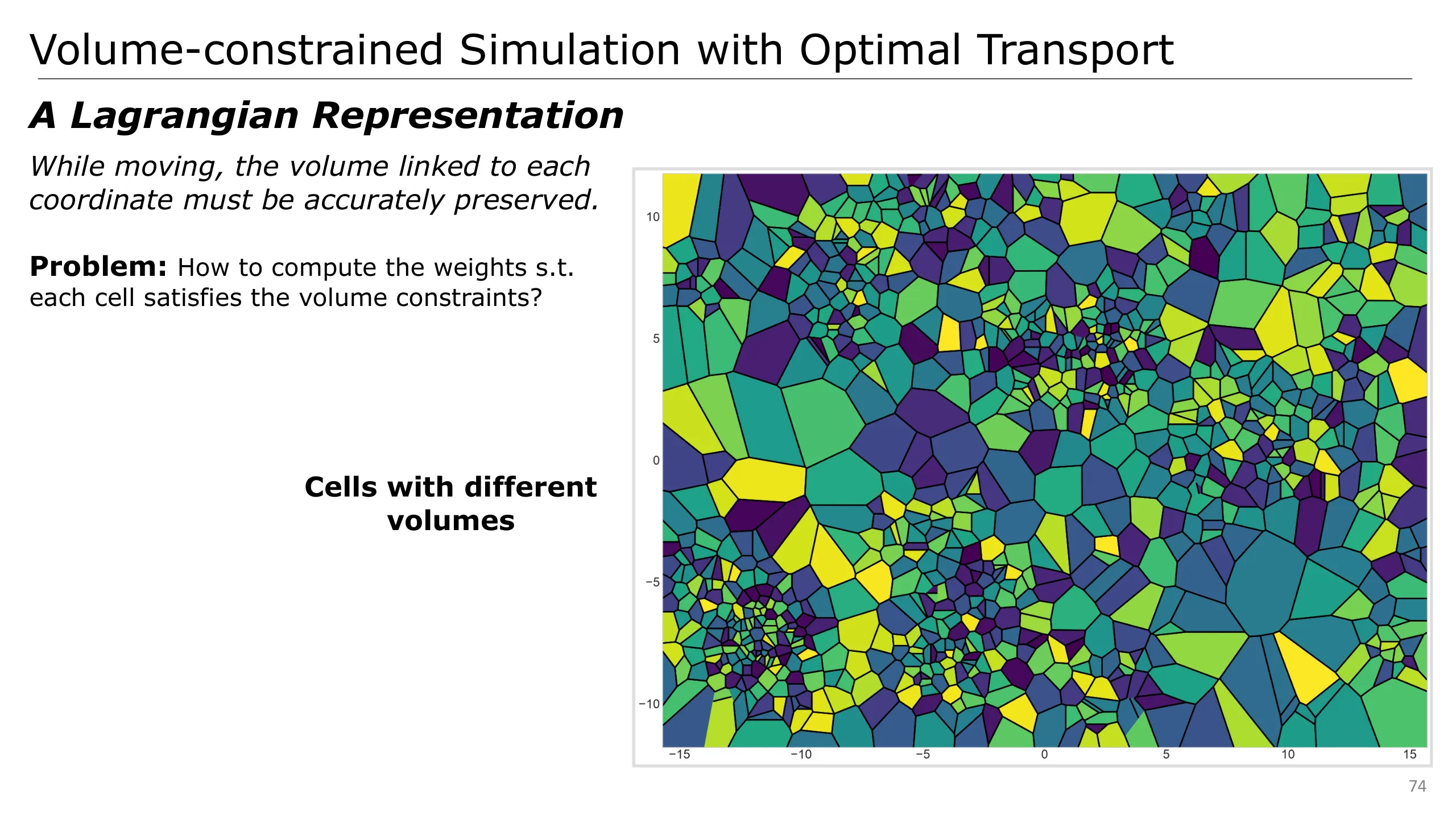
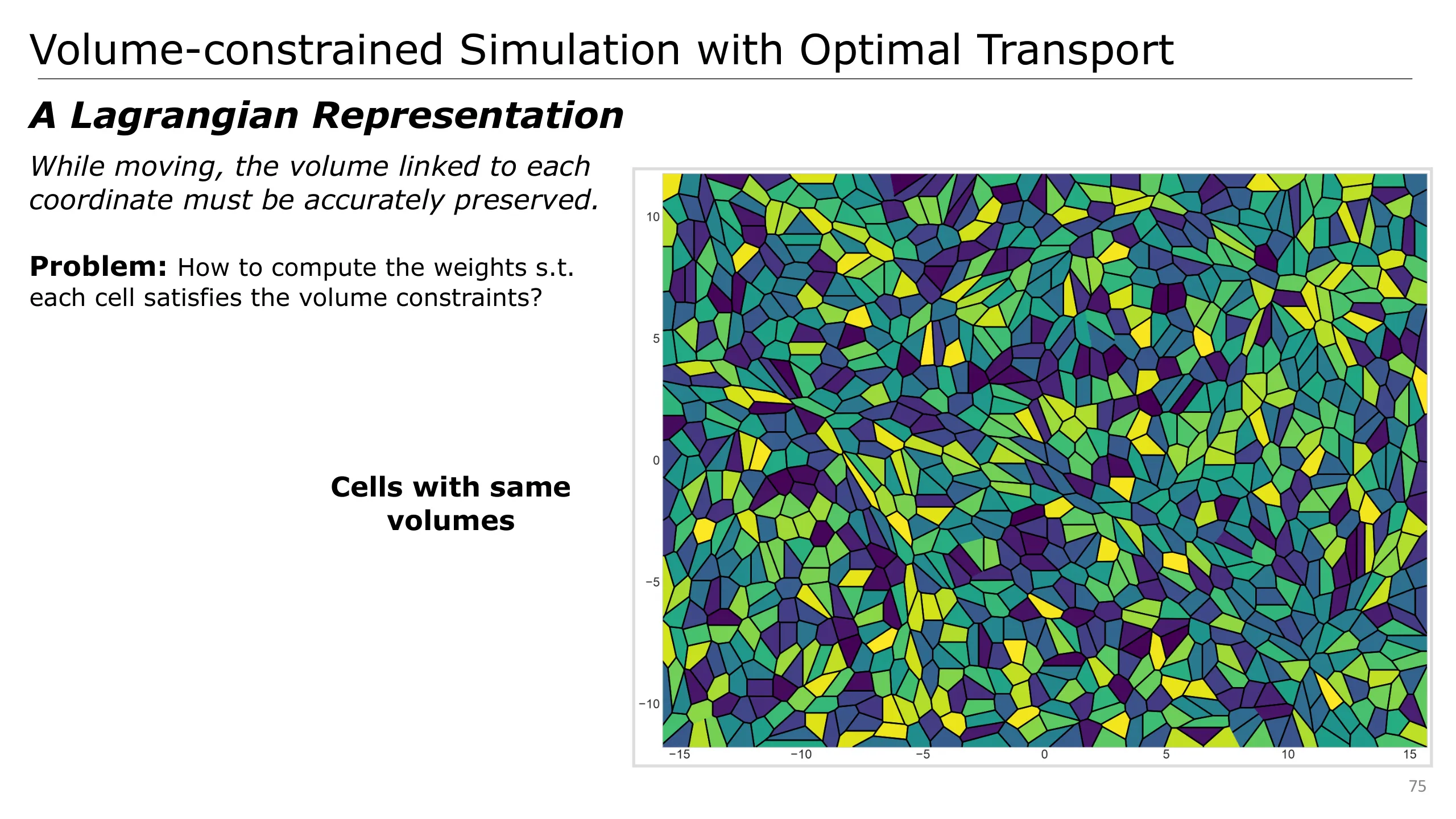
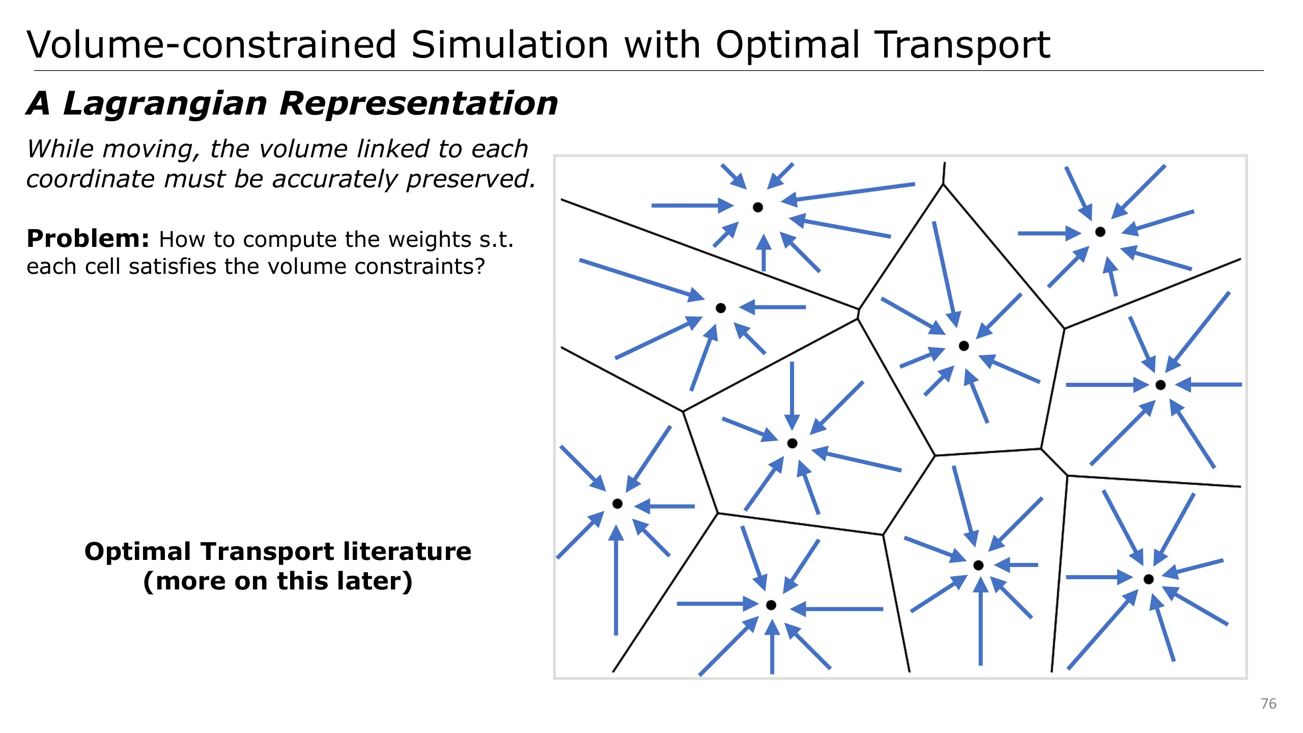
We can now wonder how to compute the set of weights s.t. each site's cell has the volume we want it to have

This is in fact a difficult problem which is directly linked to the Optimal Transport literature!

We will be able to rely on it for our problem.

We can now wonder how to compute the set of weights s.t. each site's cell has the volume we want it to have

This is in fact a difficult problem which is directly linked to the Optimal Transport literature!

We will be able to rely on it for our problem.

To see why, we will want to compute the minimisation of the moving of the matter to our Voronoi sites.

There exists a unique Laguerre Diagram satisfying the volume constraint which is the solution of an Optimal Transport problem.
This is directly an Optimal Transport problem that we will study in the next parts of this course.

Now that we have a nice representation of the geometry (i.e. a discretisation of the matter), we can consider the discretisation in time and space of its motion.

We will assume first that we have an efficient way to compute this representation (the power diagram satisfying our volume constraints) and come back to it later.

We will then focus on how to make our representation move like a fluid

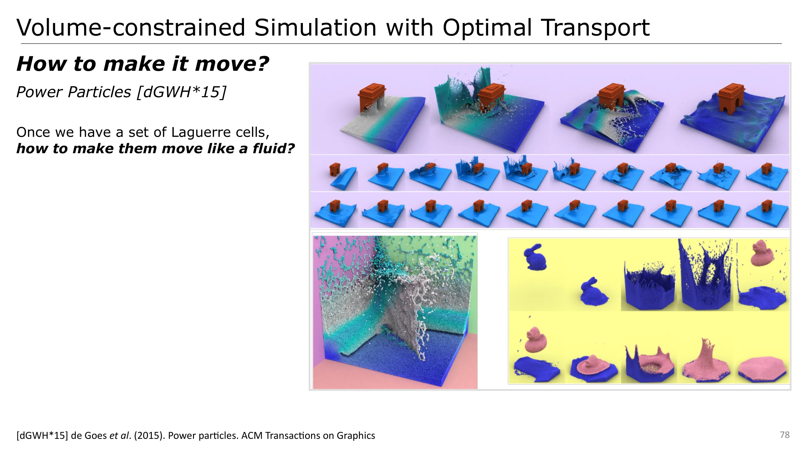
The first method actually performing this operation relying on such a representation is called Power Particles.

It is based on the idea that the volume is directly conserved over time which yields control over compressibility.

To describe how this method works, I added here first a small recap on the equations we want to discretise

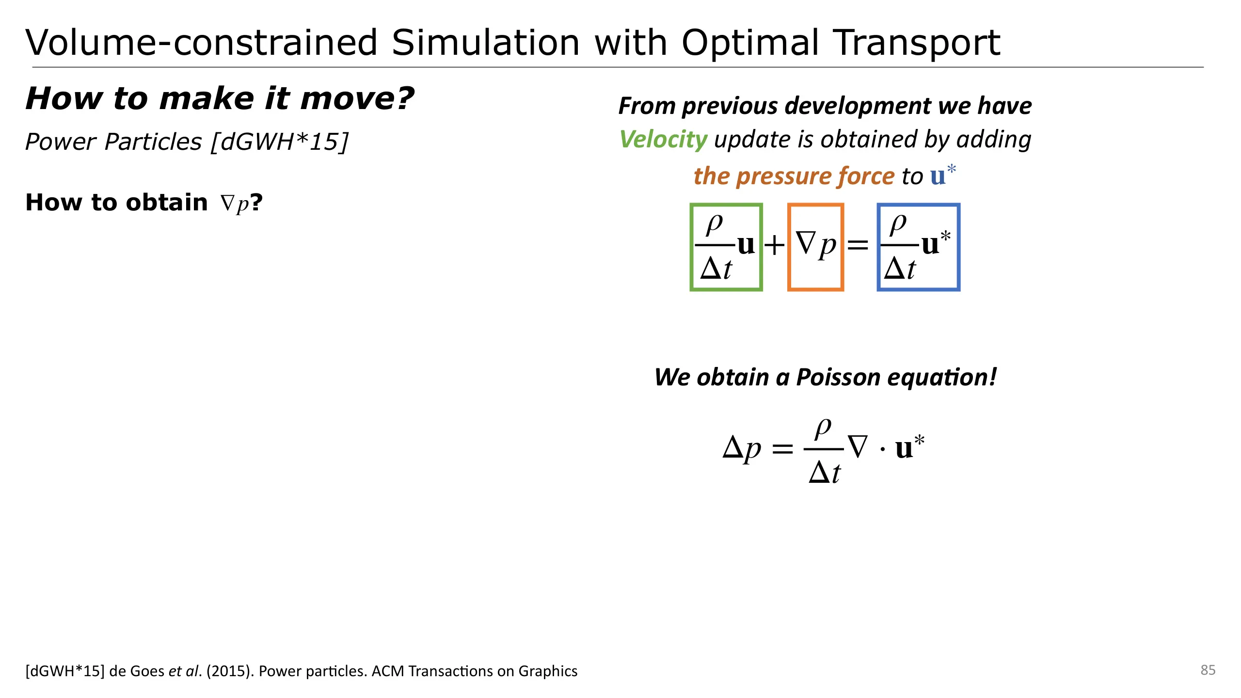
The important question is how to satisfy the incompressible constraint of the velocity field.

For that, we can consider Chorin’s method. If we rearrange the terms of our equation of motion, we have on the left side the time derivative of the velocity (i.e. the acceleration) and on the right side the pressure force and other forces.

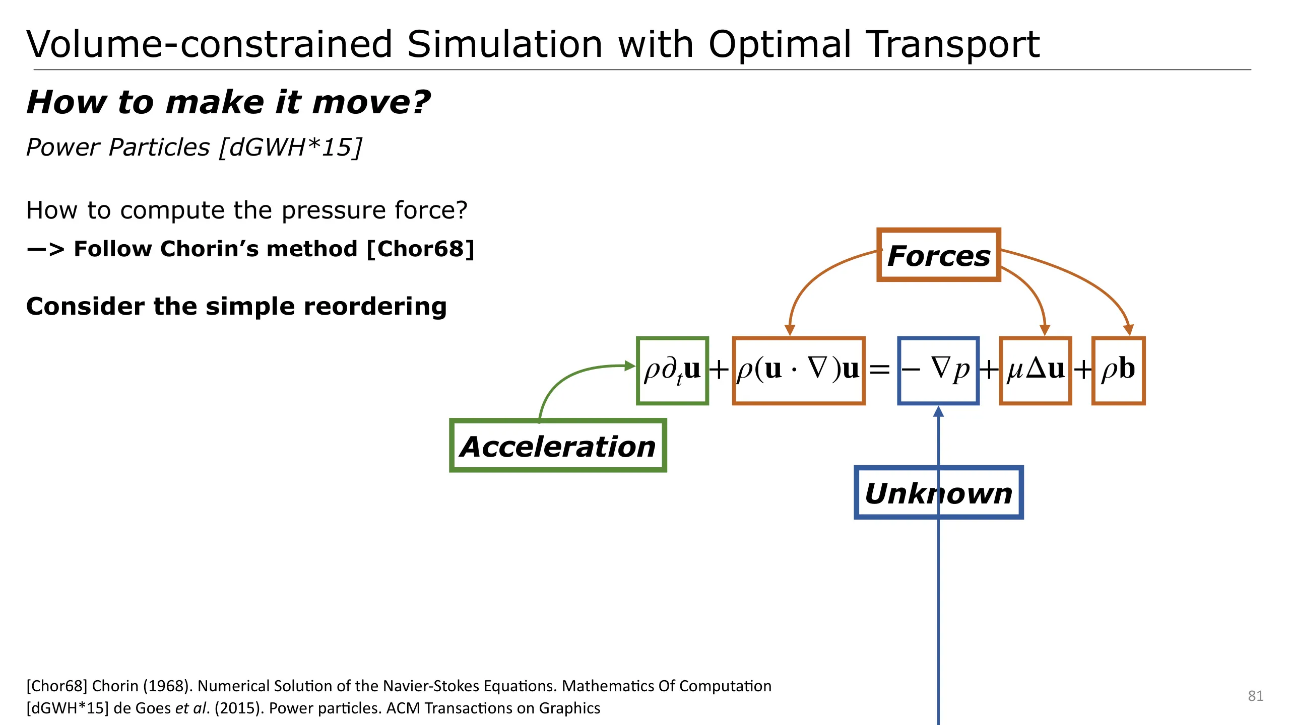
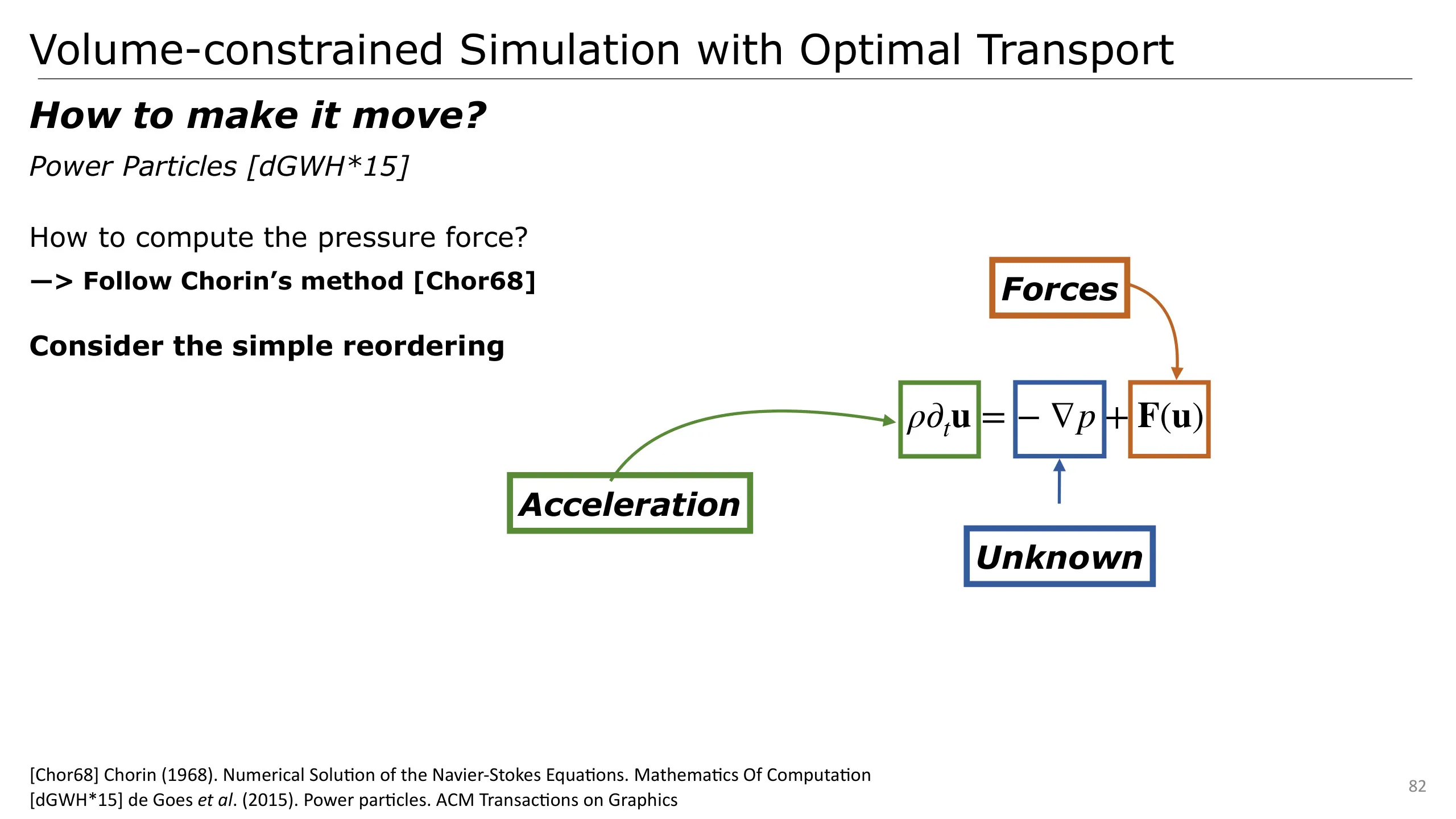
For that, we can consider Chorin’s method. If we rearrange the terms of our equation of motion, we have on the left side the time derivative of the velocity (i.e. the acceleration) and on the right side the pressure force and other forces.

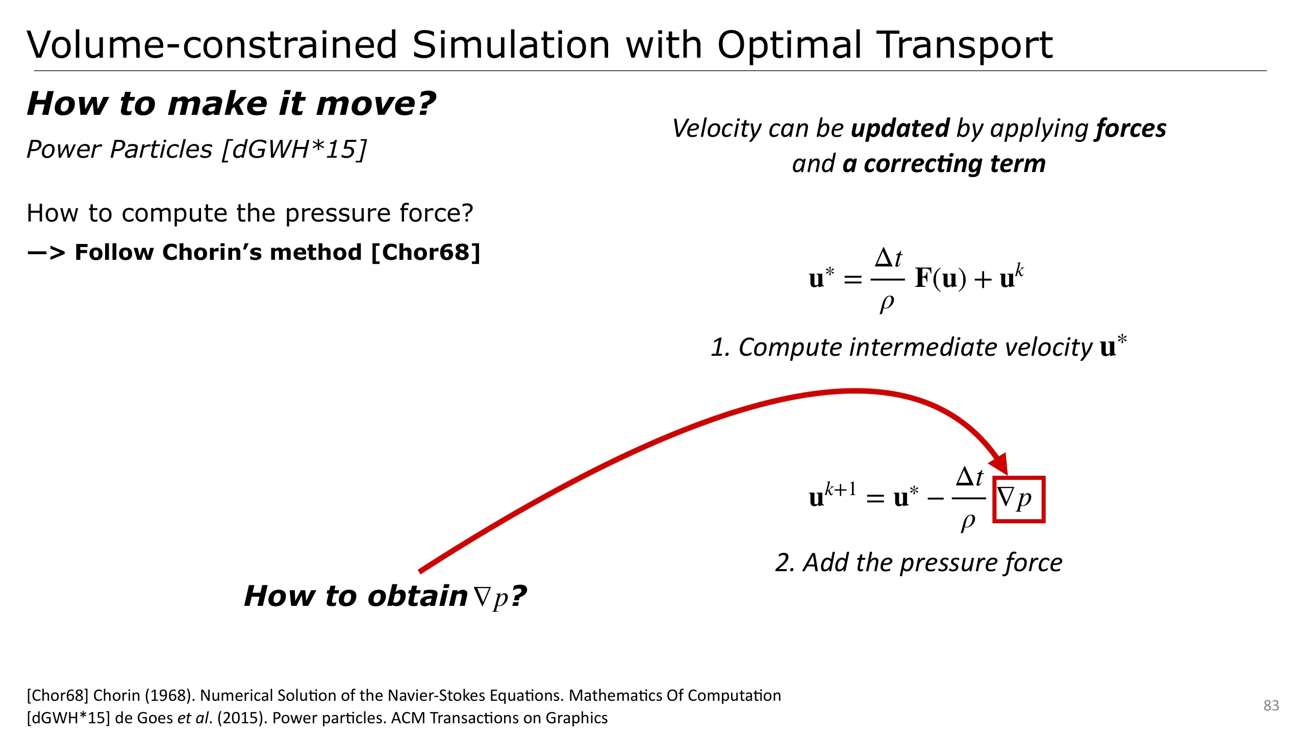
Thanks to this rearranging, we can then split the update of the velocity in two steps:

1. First, we compute an intermediate velocity by applying other forces than the pressure.
2. Second, we remove the non divergence-free part of the newly computed intermediate velocity by removing the pressure force.

The remaining question is: how to actually compute the non-divergence-free part?

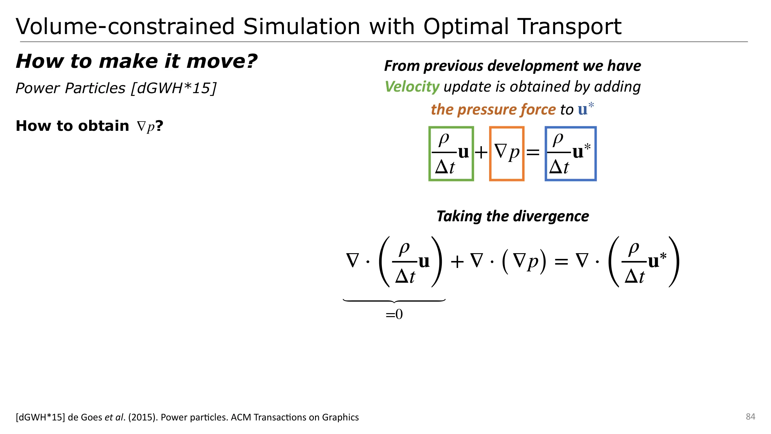
For that, we may study our equation.
It states that the difference between the intermediate velocity and the actual velocity is the pressure force.

If we take the divergence of this equation, we may notice that one term actually cancels thanks to the incompressibility constraint.

We then obtain a Poisson equation which unknown is our pressure potential p.
This is a very standard technique in CFD which is referred to as the Poisson Pressure Equation

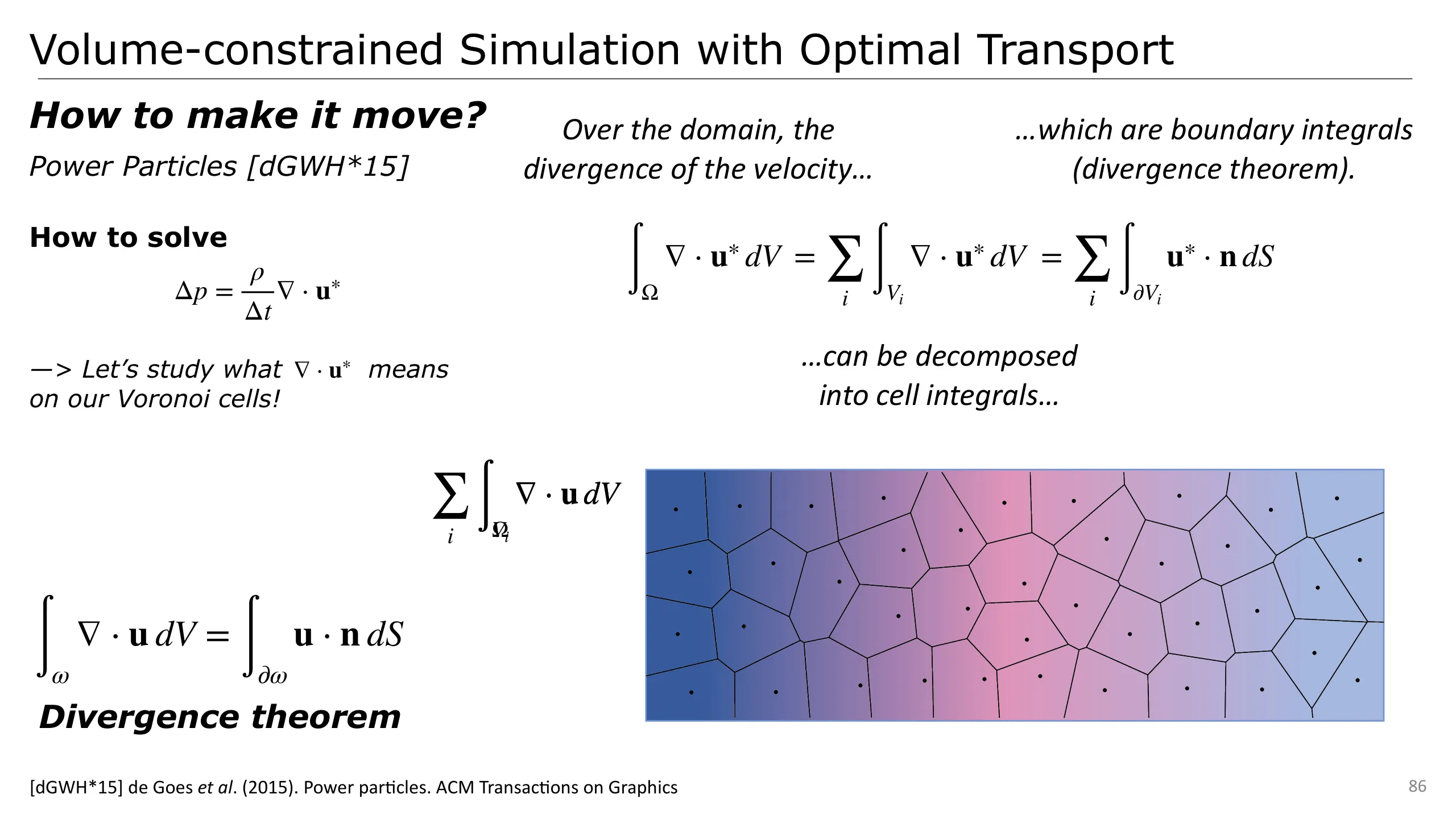
Now, to actually solve this equation, we must discretise the right term, the divergence of the velocity field.

Over the domain, the divergence of the velocity is given here and illustrated as a potential on the bottom

It can be decomposed into integrals over our Voronoi cells.

By relying on the divergence theorem given here, relating a volume integral of the divergence with a boundary integral

We obtain an integral over the boundary of our cells.

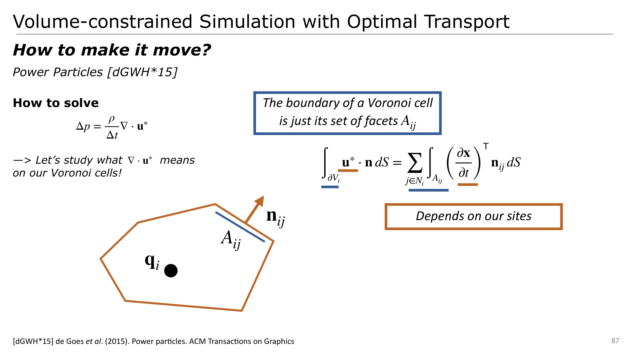
This is really nice because we can now compute its actual value!

1. And the boundary is just the sum over our Voronoi facets

2. The velocity is the time rate of change of the position on the facet which depends on the sites

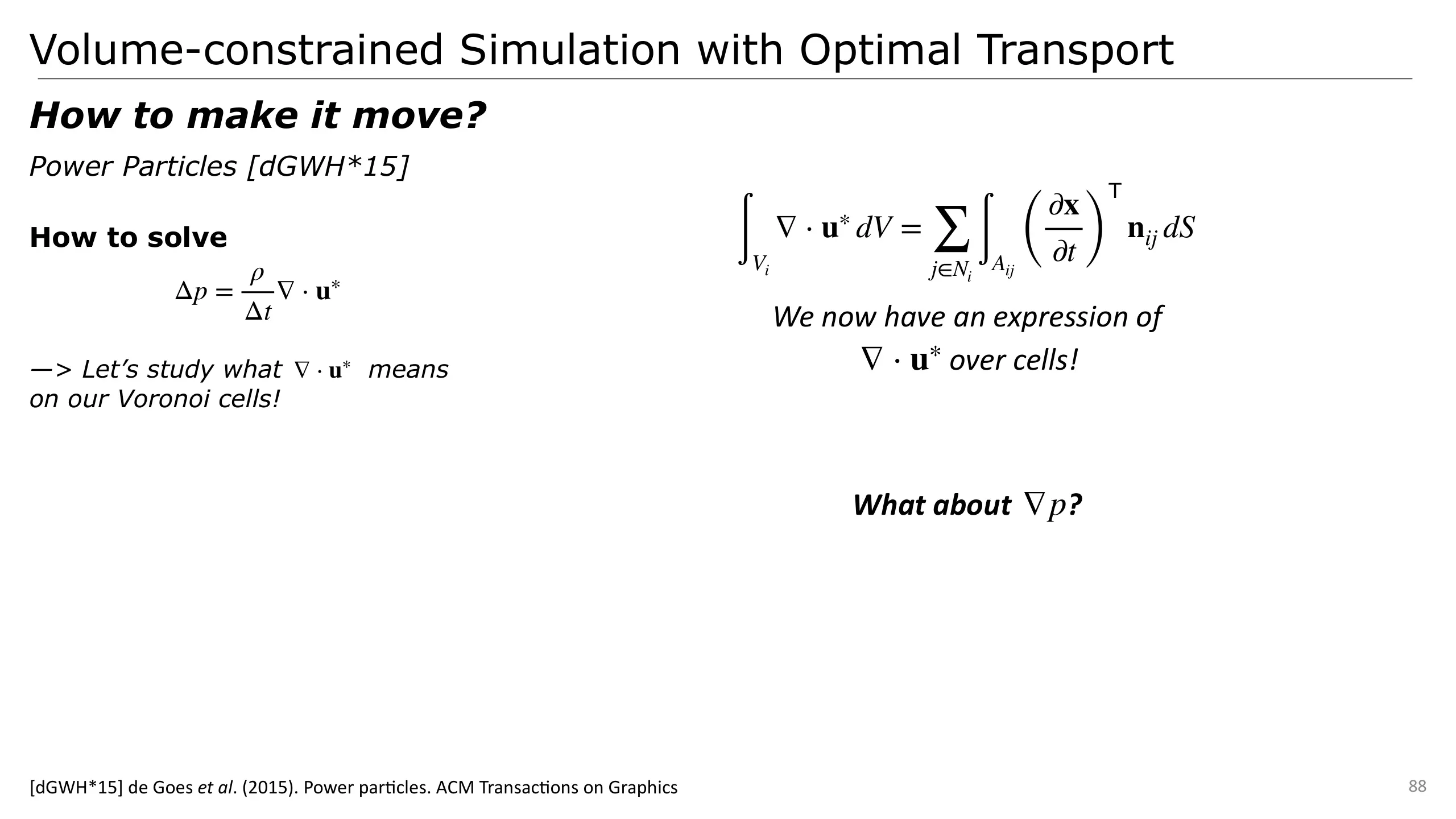
Which allows us to fully express our equation over our Voronoi cells!
However, it remains to discretise the left term of our equation, and for that we may study the gradient of the pressure.

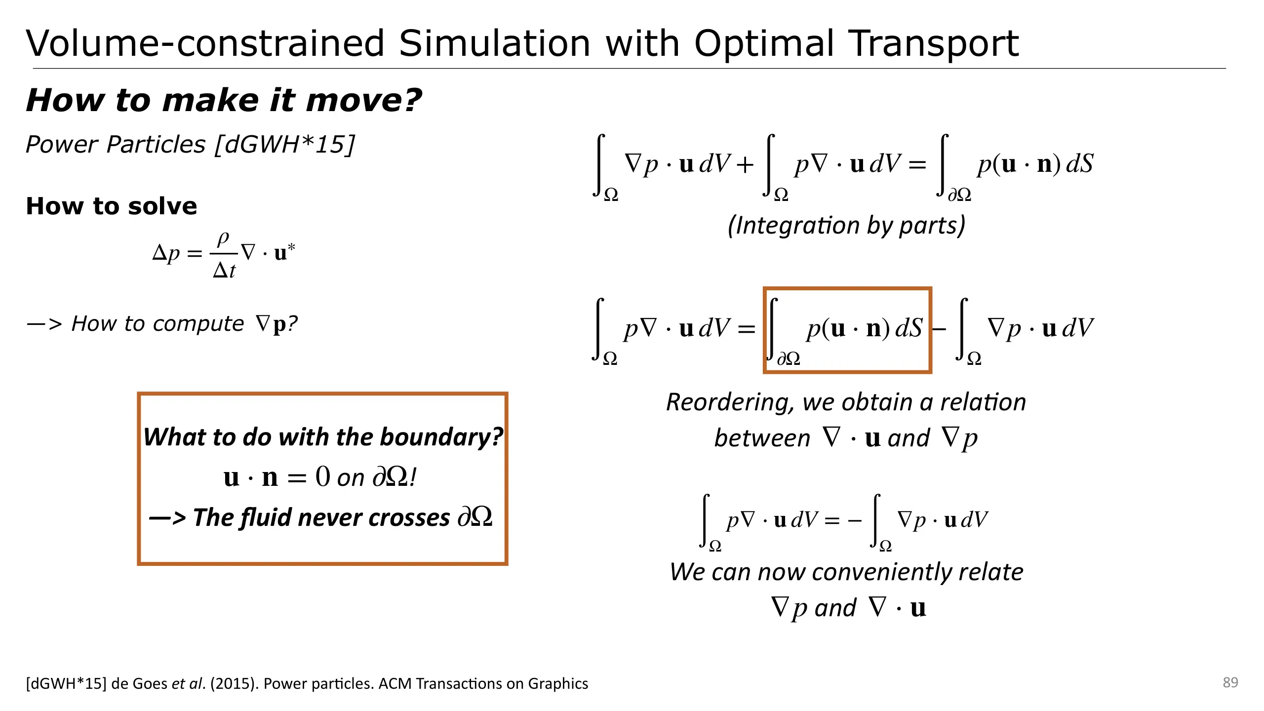
We want to compute the gradient of the pressure potential.
1. We can then rely on the integration by parts formula, which relates the gradient of a potential and the divergence of a vector field to a boundary integral.

2. By reordering, we can position on one side the divergence (that we know how to compute) and the gradient (that we’re looking for). However, it remains a boundary term that we don’t know.

3. However, our fluid actually follows some boundary conditions. On the boundary, the fluid cannot pass through it, otherwise we have a leak! This is translated into math by adding the constraint that the dot product between the velocity and the normal is equal to 0 on the boundary of the domain. This allows us to then remove our boundary term!
4. We then obtain a direct relation between the divergence that we know and the gradient of the pressure.

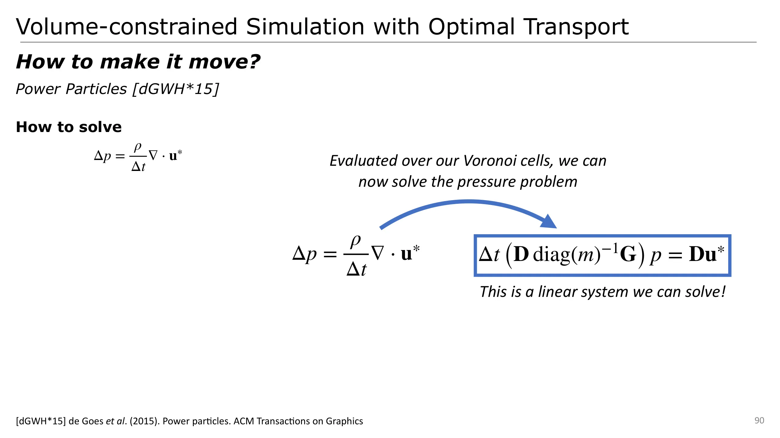
Thanks to these, we are able to define discrete equivalents of the pressure equation that we want to solve, over our Voronoi cells.

Once we know that cells can be moved from their site and how, we must actually perform the simulation.

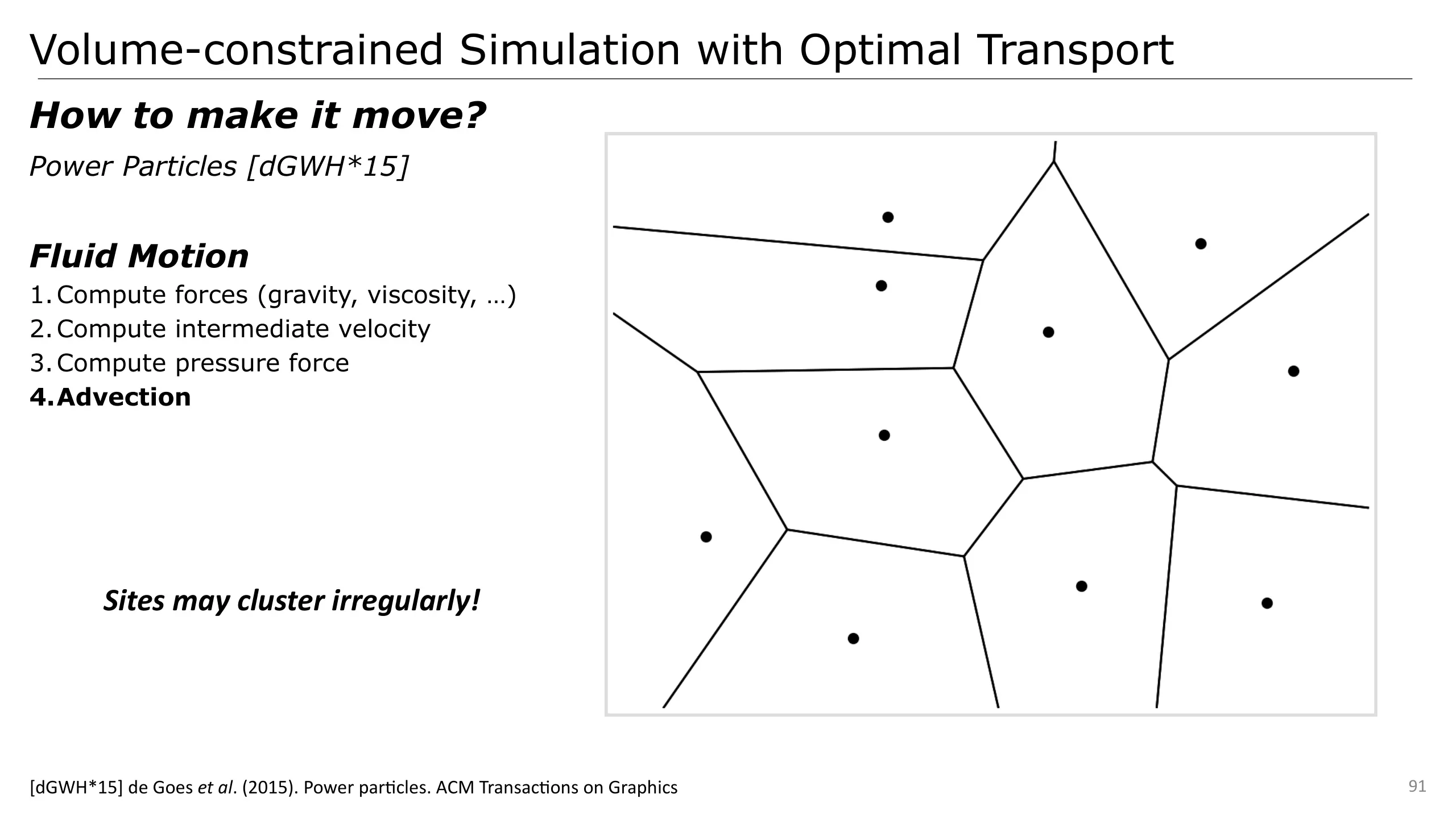
One very interesting part is the advection.

If we consider a set of sites… And its optimised Laguerre diagram…

We may want to move a site as indicated by the arrow

However, if we directly move it this way, we can see that sites may cluster.

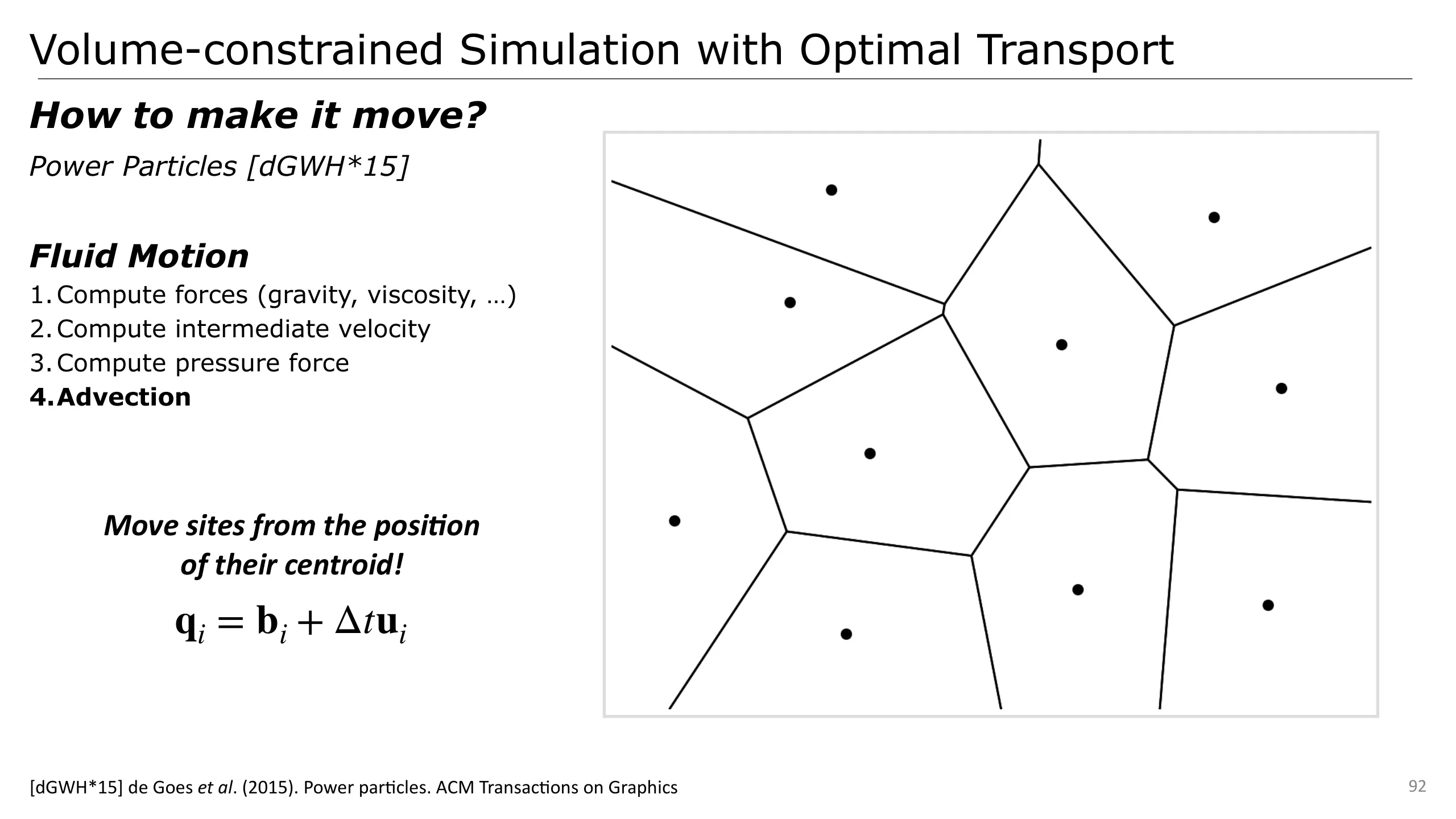
Instead, to ensure a uniformly spaced distribution of the sites, the method proposed to advect sites from the point of view of the barycentre of their cells.

We then obtain the result on the right (back and forth on animation).

We can see that sites are then well spread over the domain.

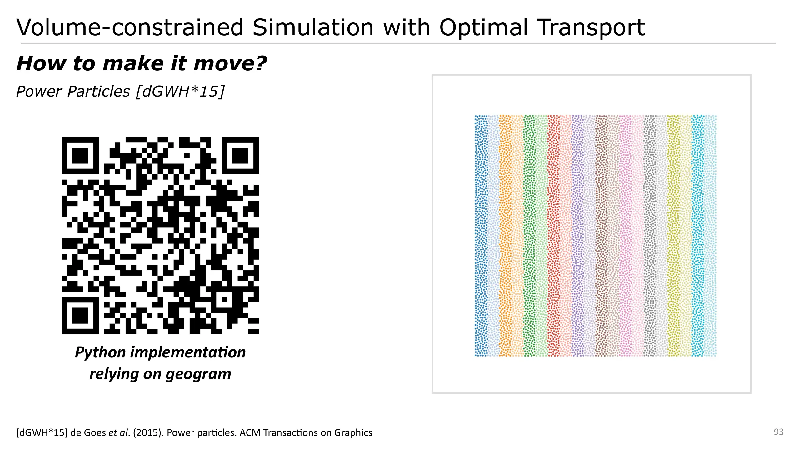
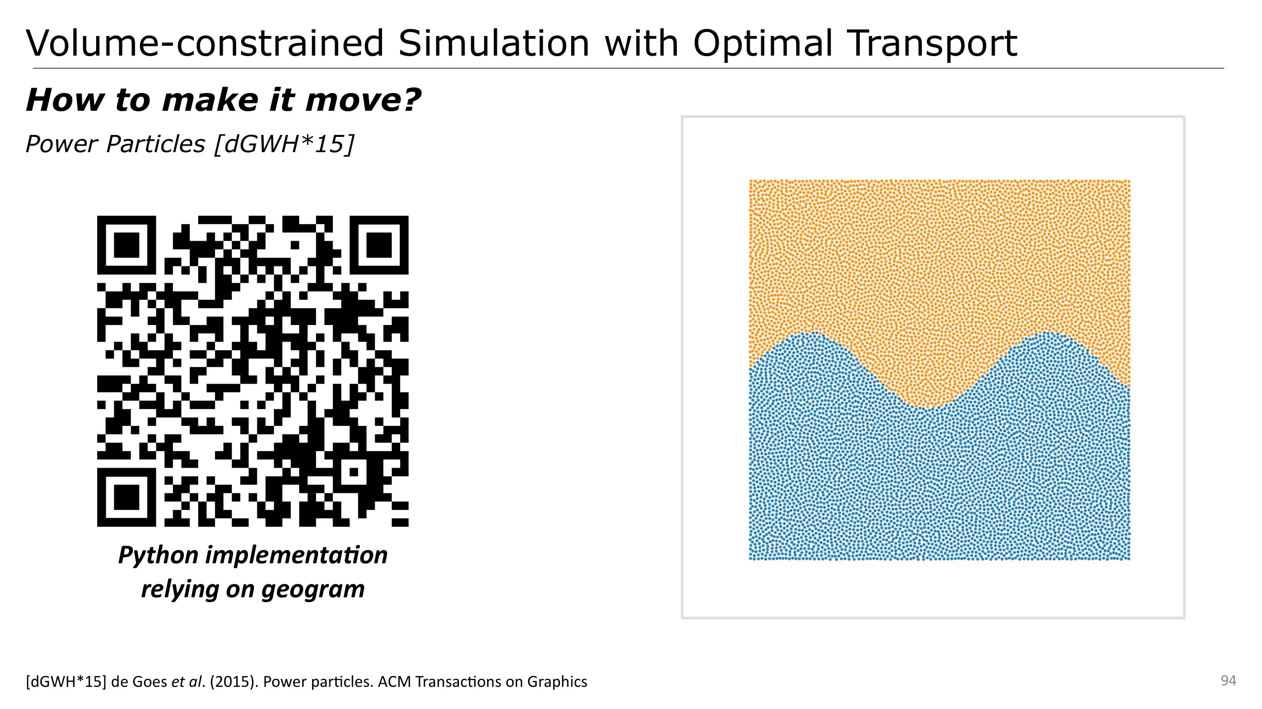
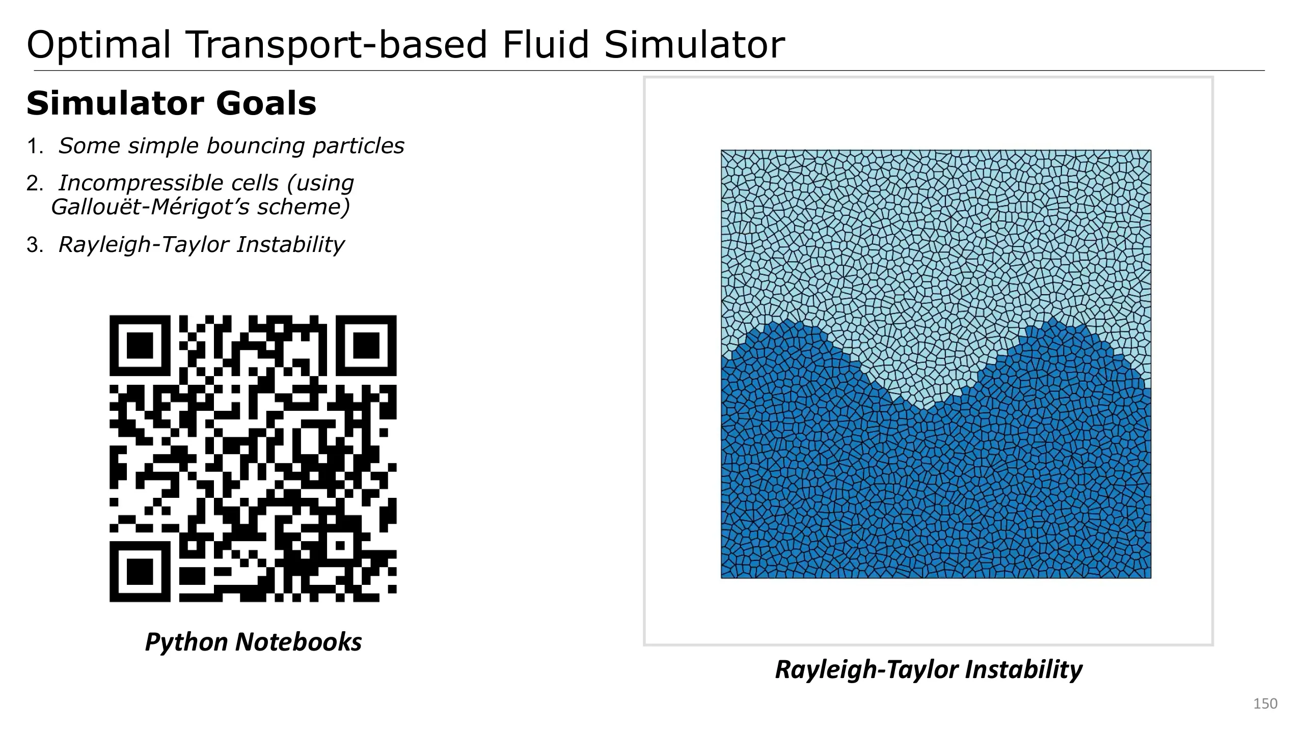
Here I’m showing some examples that I have implemented in Python relying on geogram.
First, we have these Taylor-Green vortices.

And here the Rayleigh Taylor instability. Here, the orange fluid is denser than the blue one.

Finally, here are more complex results by de Goes et al. relying on 600k fluid particles, the method yields good results even at large scale.

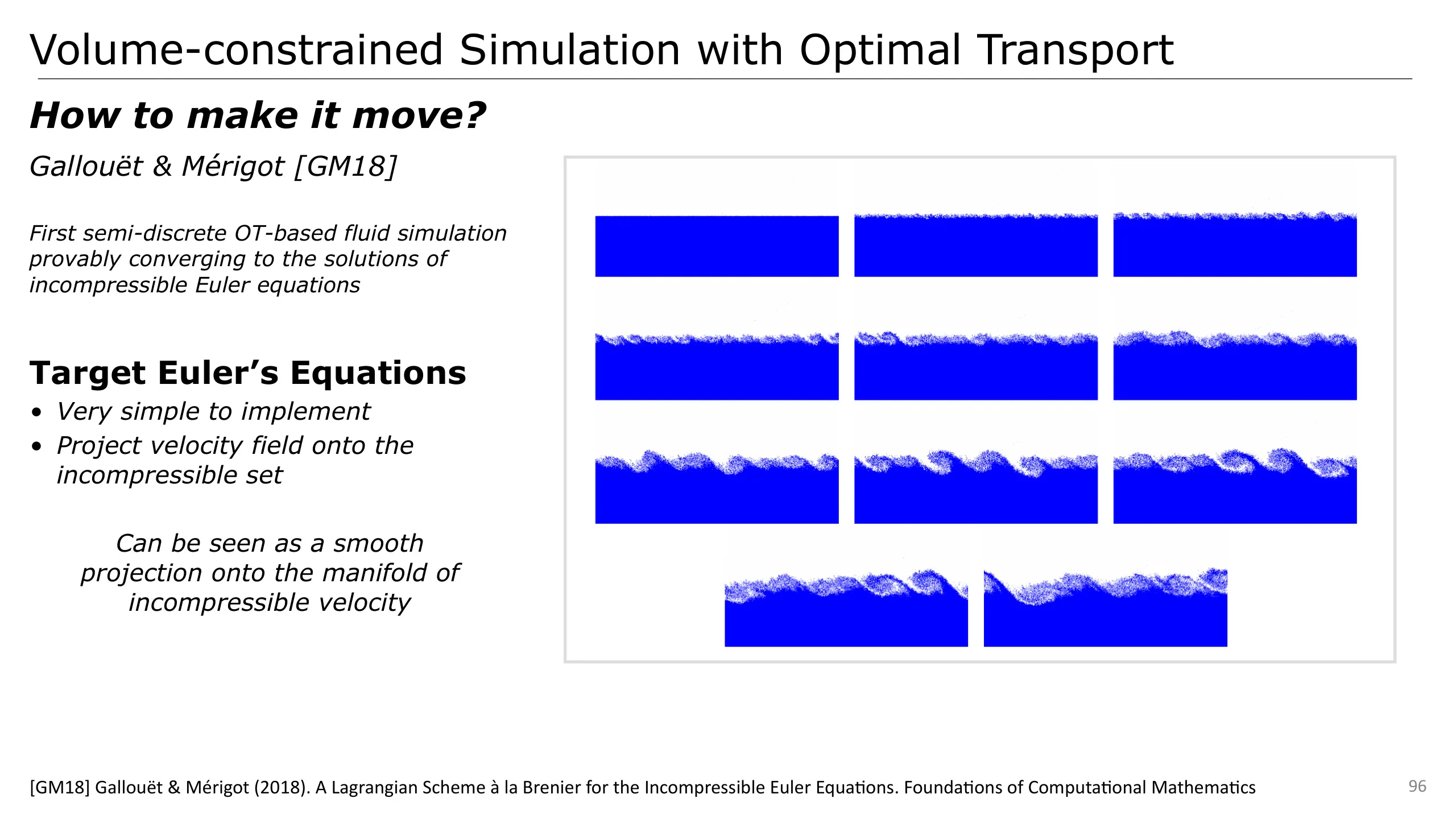
An alternative method has been proposed by Gallouët and Mérigot in 2018.

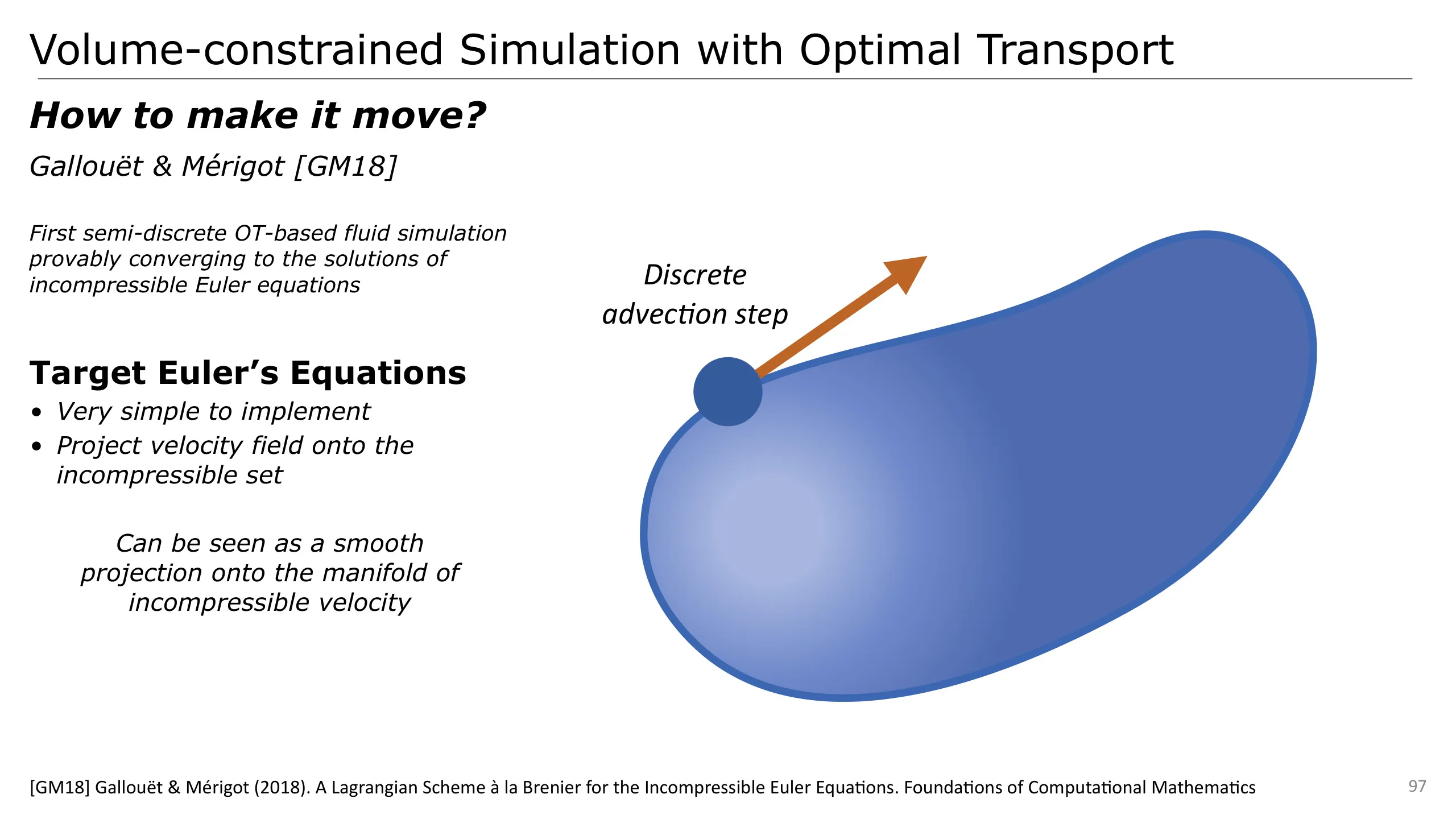
Their goal was to provide a discretisation provably converging to the incompressible Euler equations.

These are a specific case of Navier-Stokes equations, where there is no viscosity force.

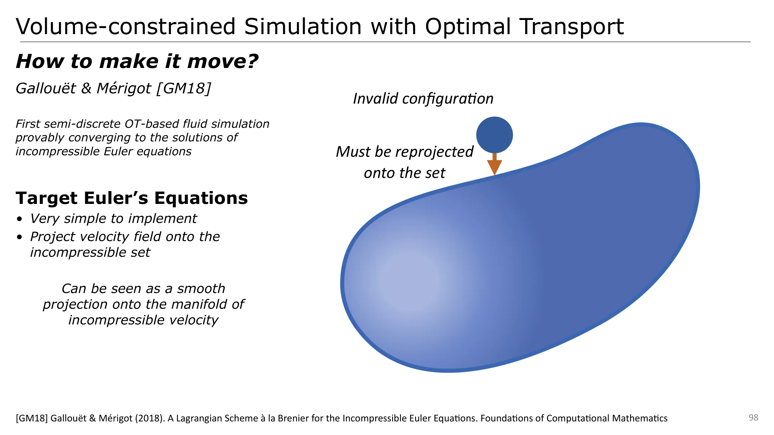
For that, they rely on Arnold’s point of view of incompressible fluid which considers them as geodesics on the manifold of incompressible motion.

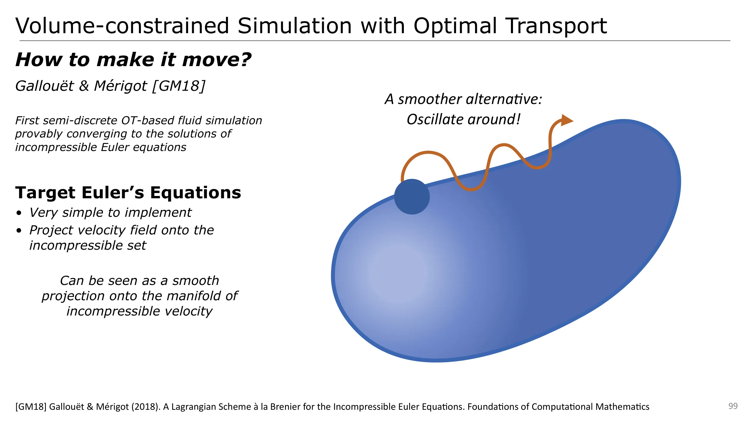
I’m representing the current motion configuration state as a point on this manifold on this schema.

While discretizing the motion, we make a small error taking us out of this manifold.

To ensure that we remain on it, we have to reproject onto the manifold.

This is actually what we did for the power particles’ method by solving the pressure force.

An alternative method, proposed by Brenier is to perform a smooth oscillation around the manifold of incompressible motion.

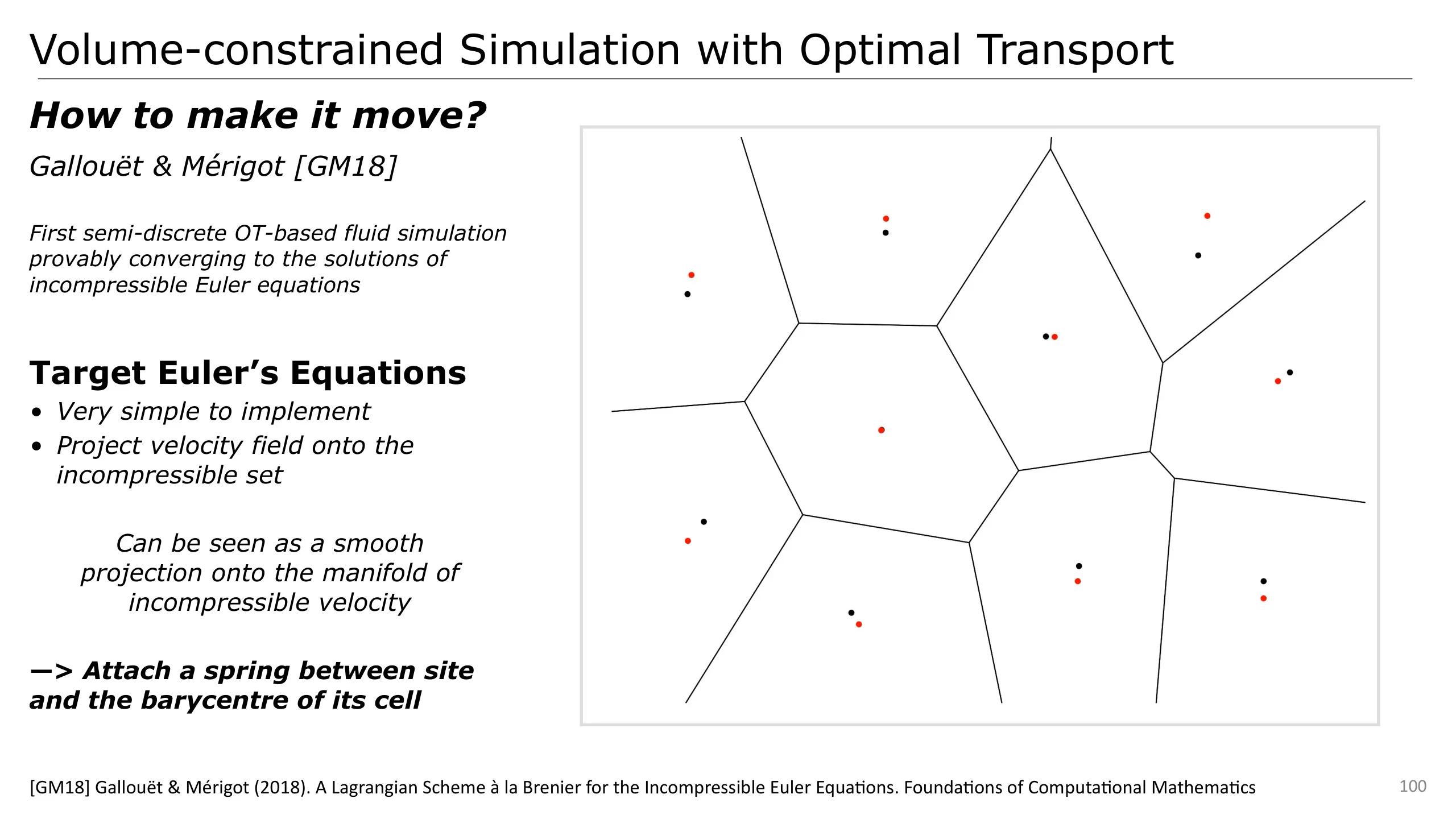
To actually perform this oscillation, Gallouët & Mérigot follow Brenier’s method by attaching a spring between the site and its barycentre.

I’m illustrating this on this unnatural setup which highlights the motion. Sites are represented in black and centroid in red.

We can see that the sites oscillate around their centroid.

A sharp difference between this scheme and de Goes et al.’s scheme is that this one couples the geometry and the physical energy.

The physical energy is obtained as a function of the minimized geometrical energy

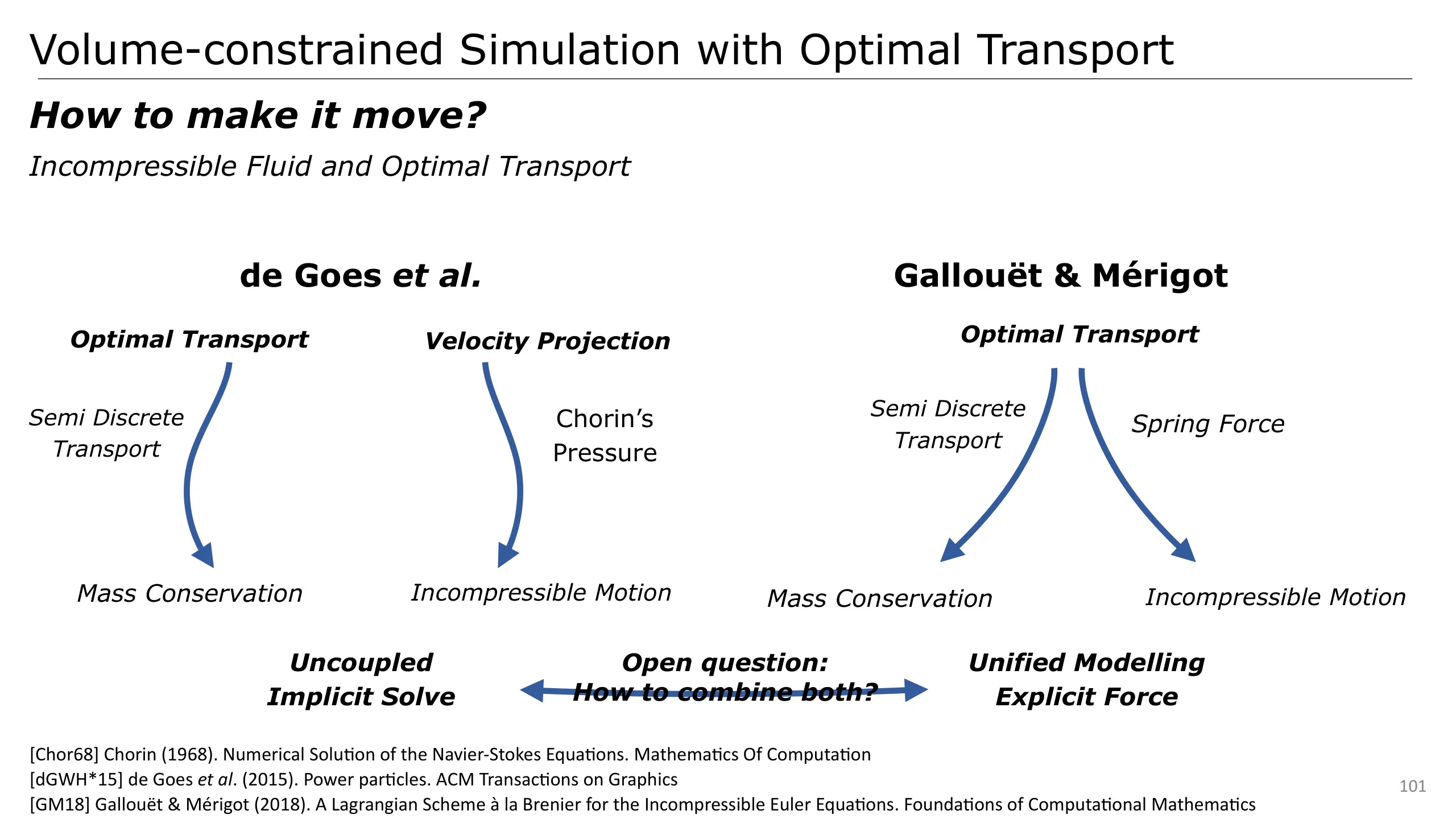
Now that we have seen these two methods, we may wonder why they compute pressure so differently and what are the advantages and drawbacks of both methods.

First, de Goes et al. decouple OT and Pressure solve. Both handle two different sides of the incompressible fluid problem: one gives the mass conservation while the other provides the incompressible motion.

On the other hand, Gallouët & Mérigot rely on OT for both Mass Conservation and derive an incompressible motion through an explicit force given by the OT problem.

We then have on one side an implicit solve offering physical parameters and robustness to large time steps or resolution changes but in an uncoupled way.

On the other side, we obtain a unified modelling through an explicit force which however requires an additional parameter and is depending on resolution

This lets us highlight an open question: How to combine the advantages of both strategies?

Based on these approaches, multiple works introduced additional effects relying on this discretisation.

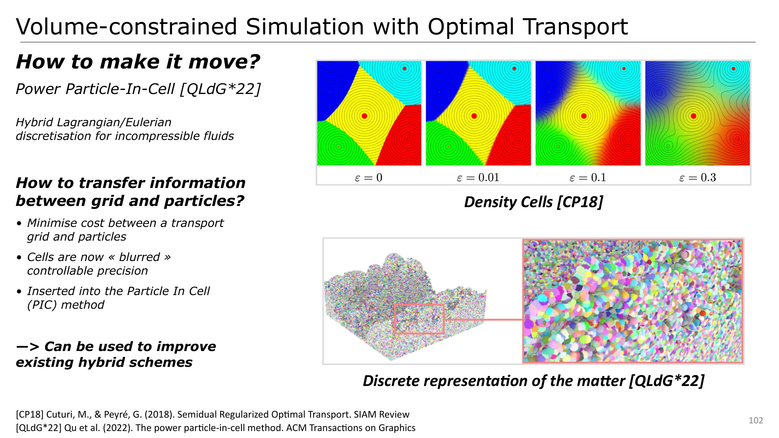
Qu et al. rely on this representation as a way to make hybrid schemes more robust.

One of the problems is these methods can lose some volume of matter over time and particles may cluster.

To address these issues, Qu et al. consider some Lagrangian particles coupled with a density kernel.

To insert this into the framework we just discussed and benefit from its characteristics, they rely on a generalisation of Laguerre cells.

Instead of considering sharp cells, they instead follow the work of Cuturi and Peyré who rely on densities.

Cells are now blurred which leads to efficient discrete algorithms, referred to as entropy regularised Optimal Transport.

Once this optimal transport problem solved, cells are directly mapped to a grid which directly describes the occupancy of the fluid.

The transfer to the Eulerian grid can be made efficiently since we already assigned parts of the Eulerian space with the Lagrangian particles

This improves significantly existing hybrid schemes with additional guarantee on mass conservation.

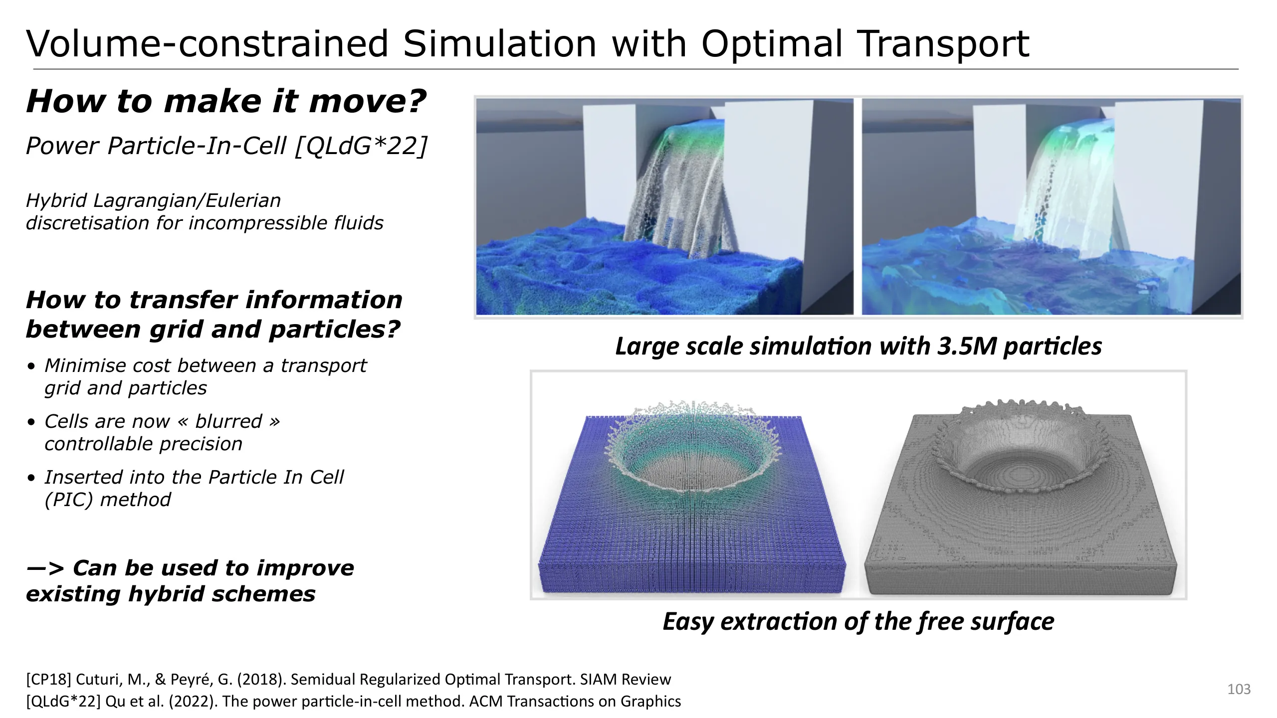
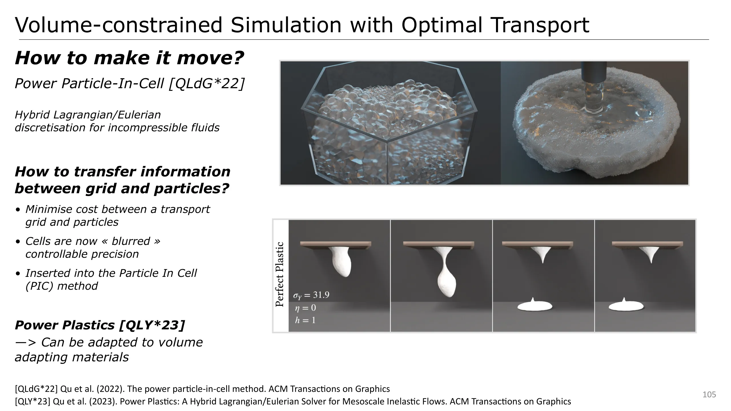
Authors have shown that, thanks to the efficiency of their method, large scale simulation can be performed as shown on the top right.

Additionally, since we directly have a background grid, we can easily extract a free surface geometry for rendering purposes.

Here I’m showing some results by Qu et al.

This work has also received follow-ups for mesoscopic inelastic materials like bubbles and foams with impressive results!

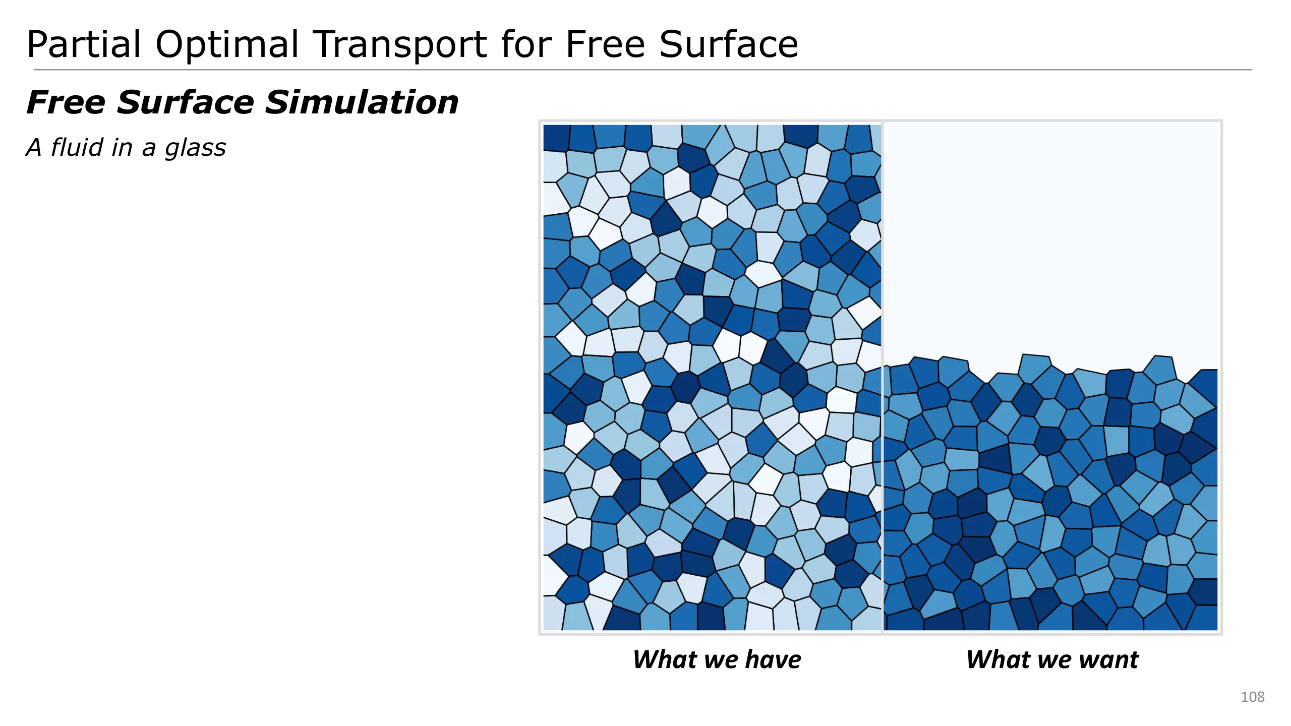
The Optimal Transport problem we study up to here fully fills the domain.

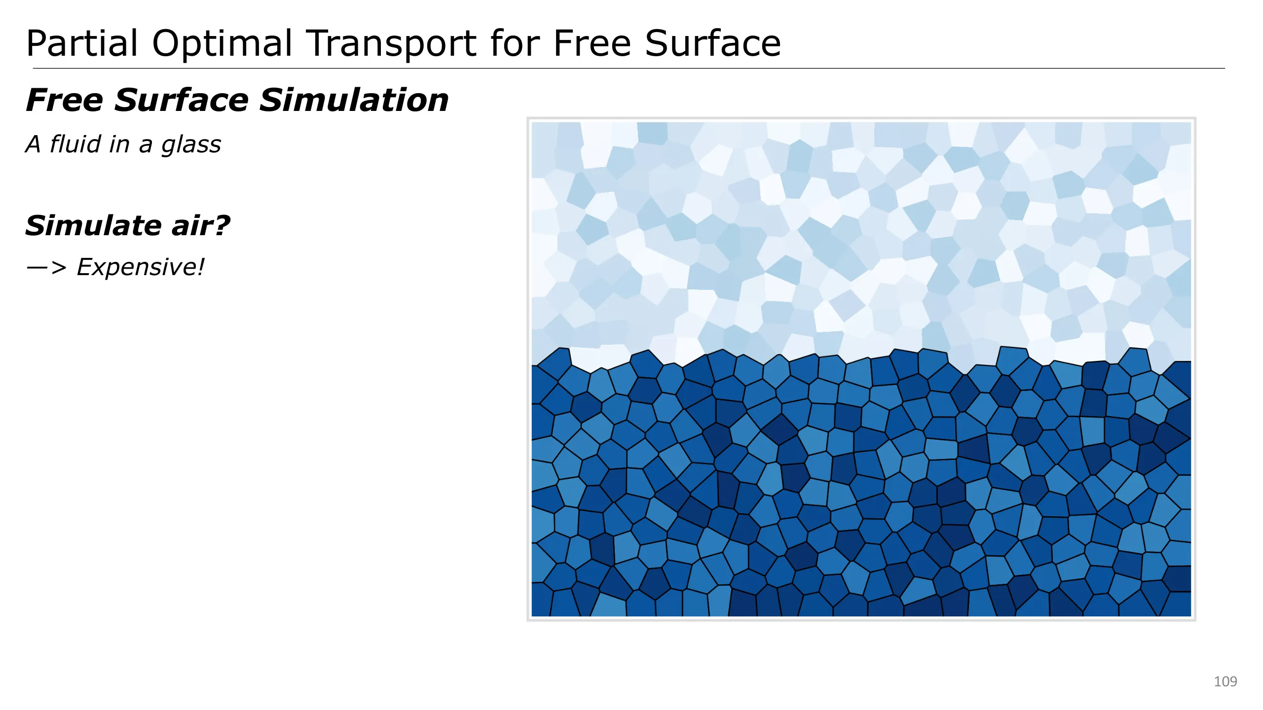
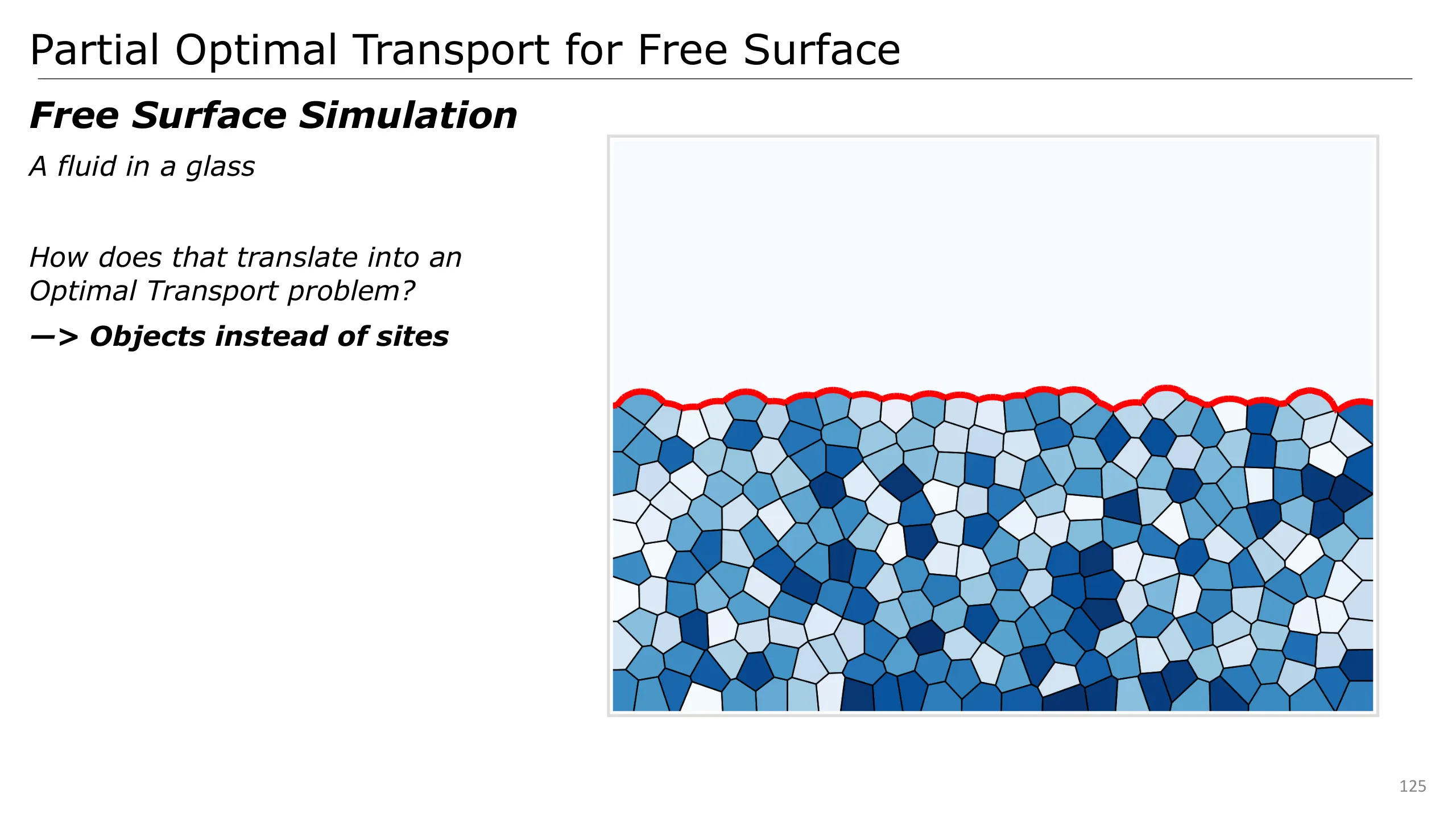
However, we may want to simulate a fluid that occupies a smaller part of the domain as the figure on the right, which is called a free surface fluid.

This way, we could simulate splashes and droplets in a glass of water!

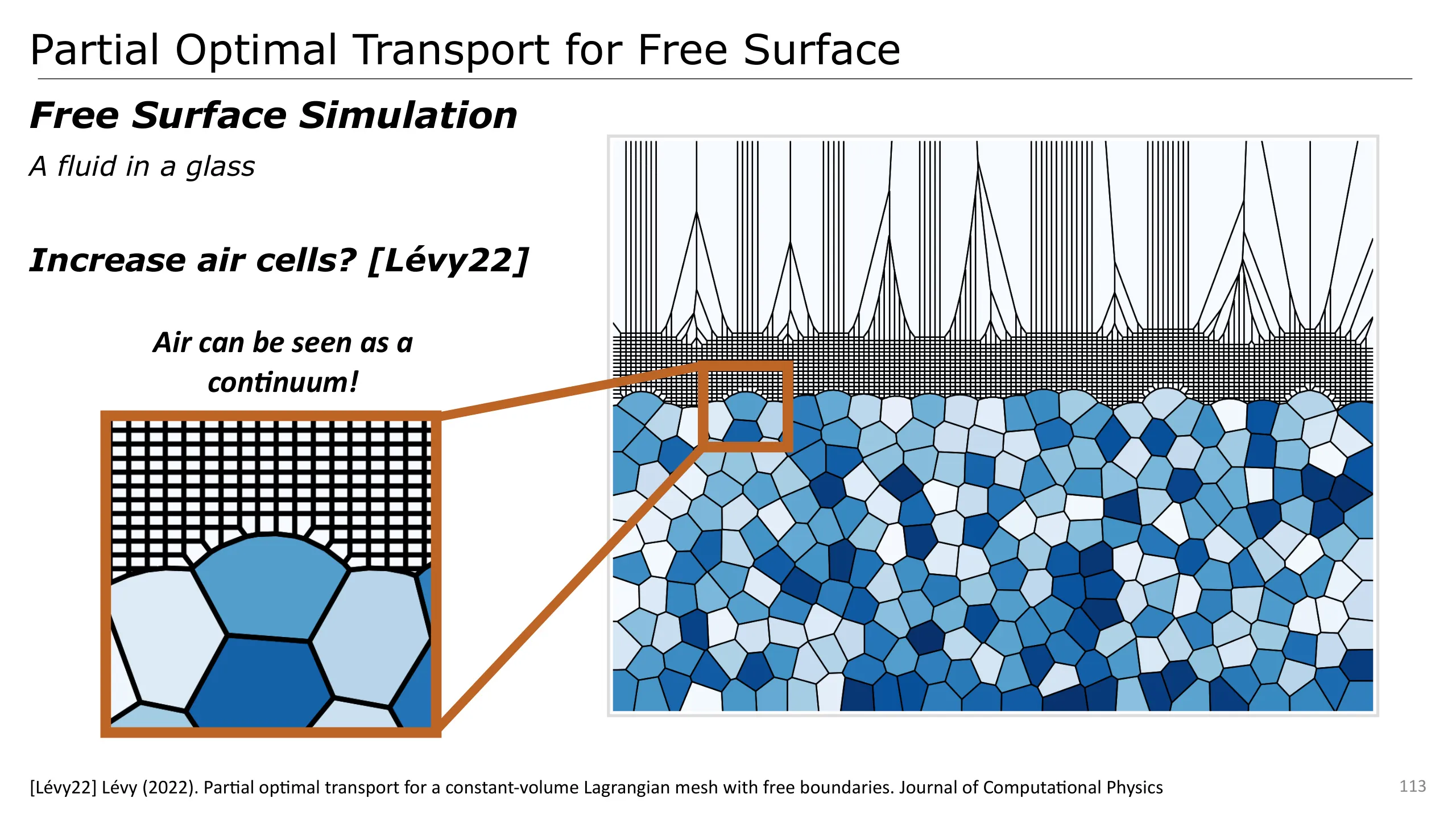
What we can do to do that is to add some cells representing the air, but that is very expensive since we are simulating two fluids.

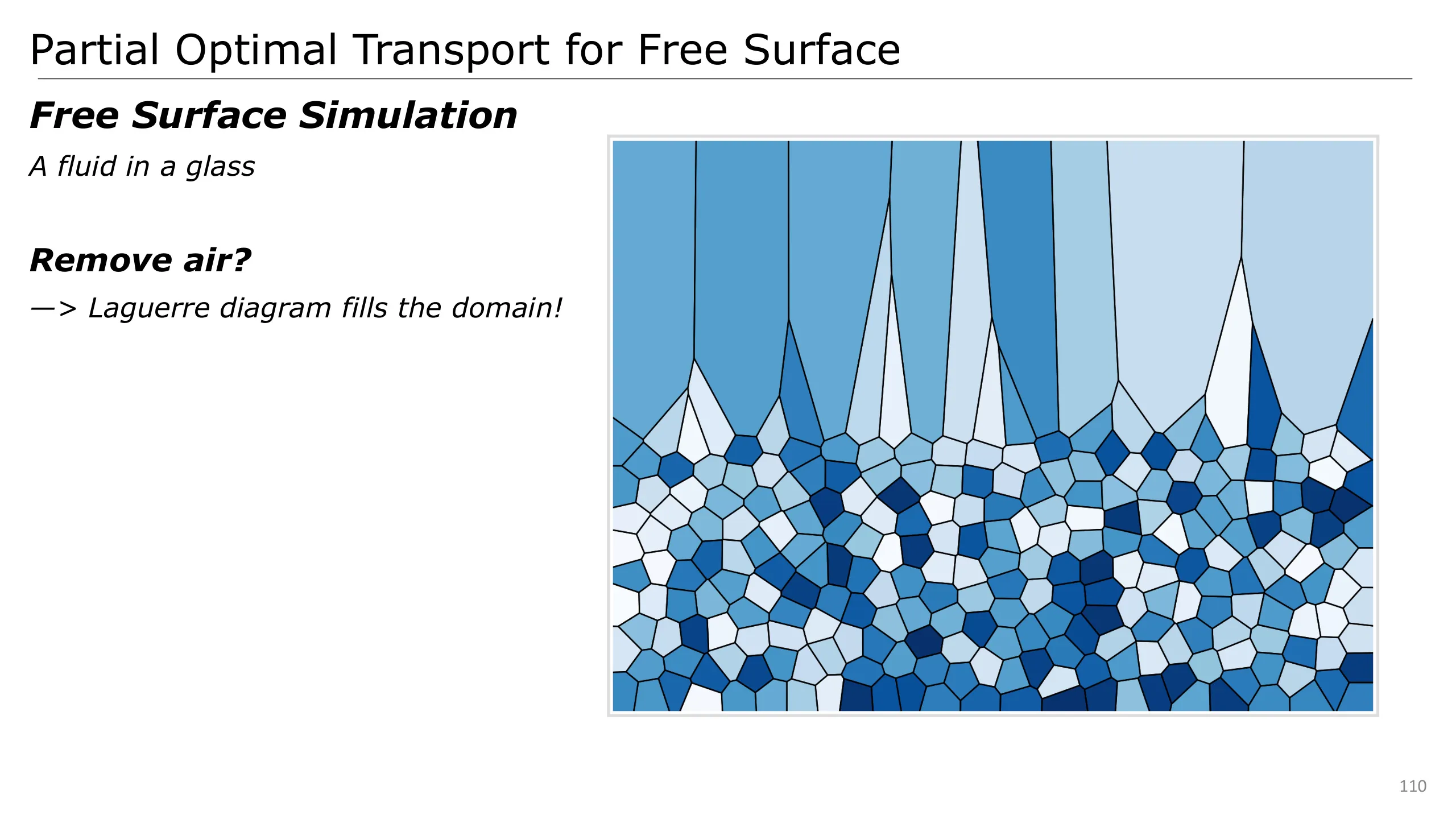
We can instead consider just removing air, but the Laguerre diagram is a tessellation of the space. We will not be able to restrict it to the subvolume of the domain we wish for our fluid.

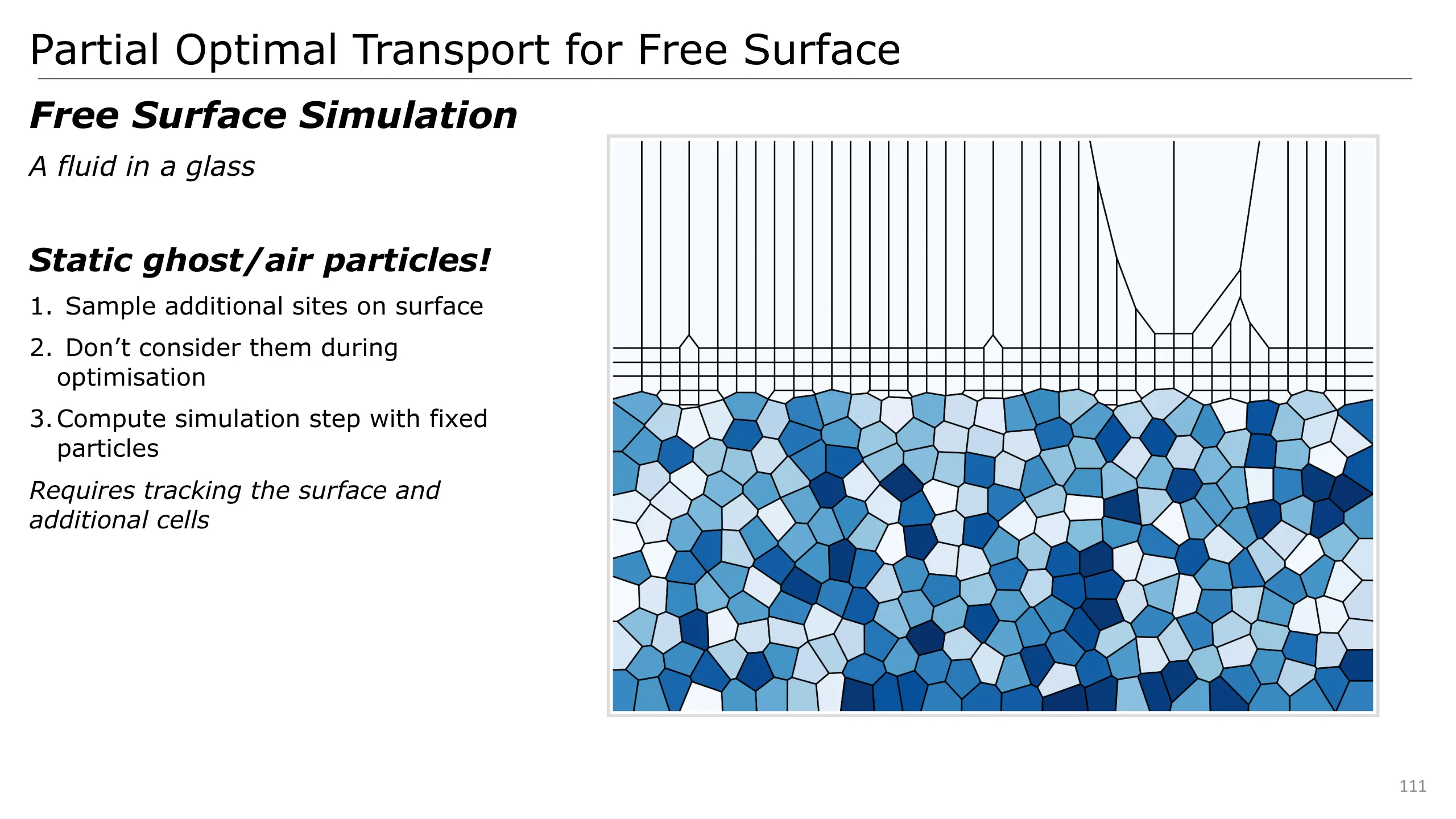
Instead, de Goes et al. proposed to sample some air particles in a limited area around cells of the surface.

Assign them a portion of the air.

And compute the simulation step while fixing the position of these air particles.

This considerably reduces the cost of air particles, but still leads to additional processing.

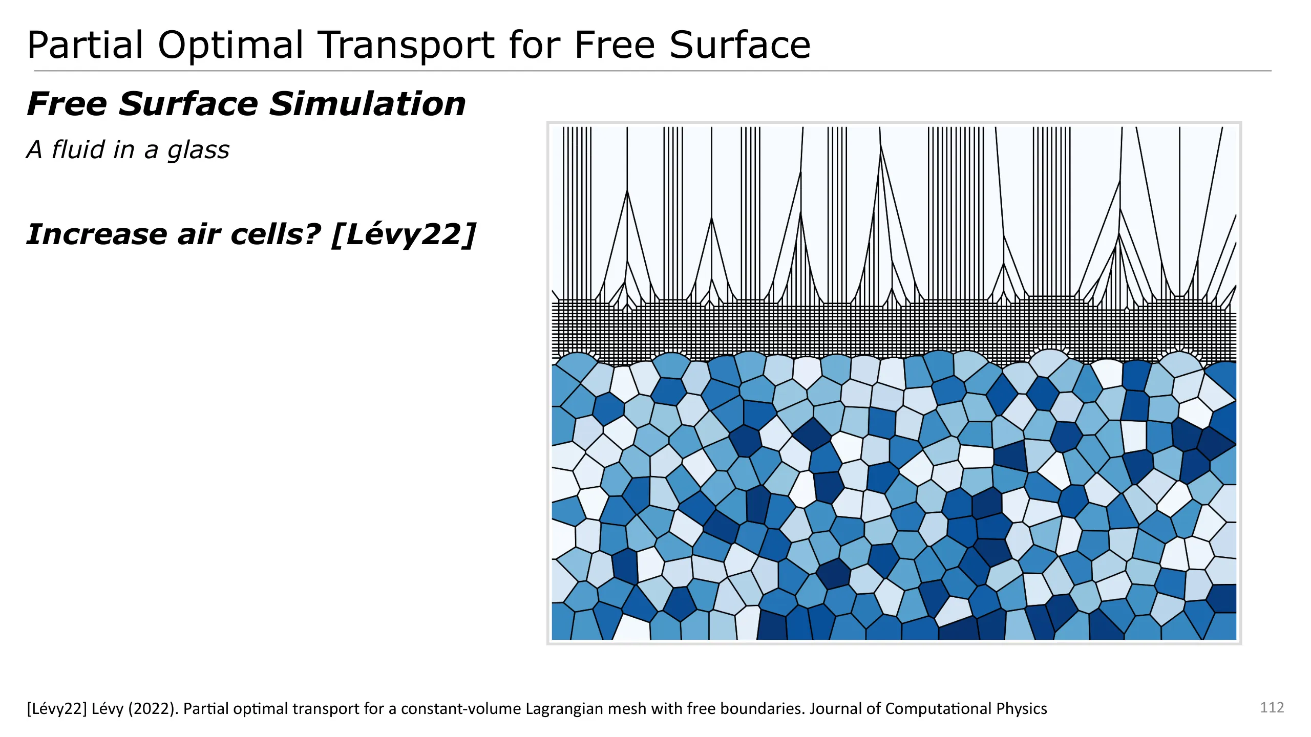
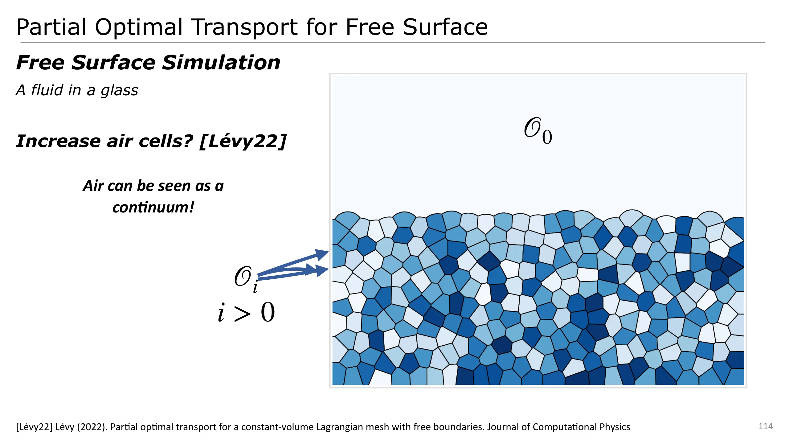
Instead, we can take the opposite point of view and increase the number of air cells.

As we can see there is a pattern. To better study it, we can take one step further and consider ghost cells as a continuum.

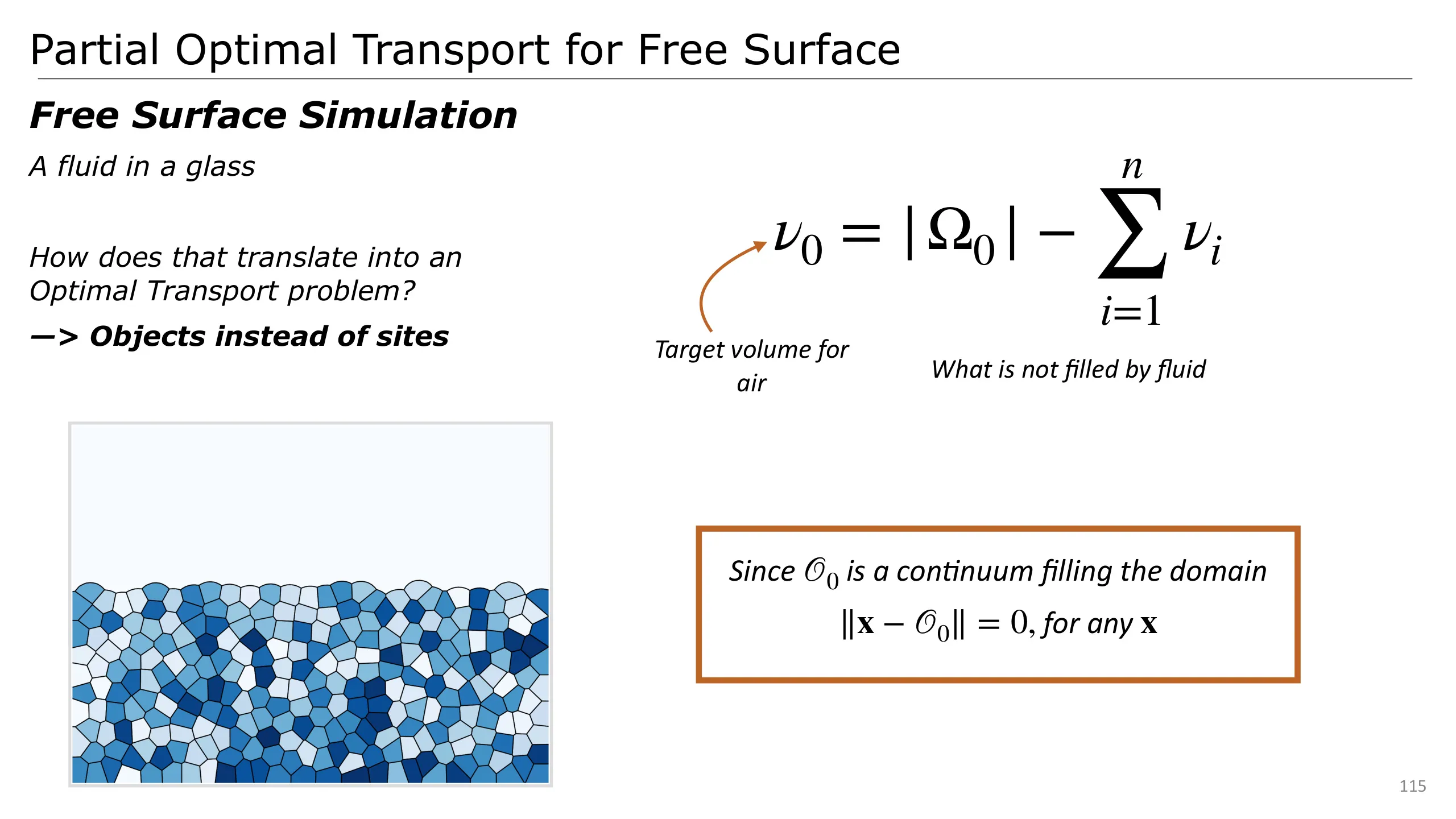
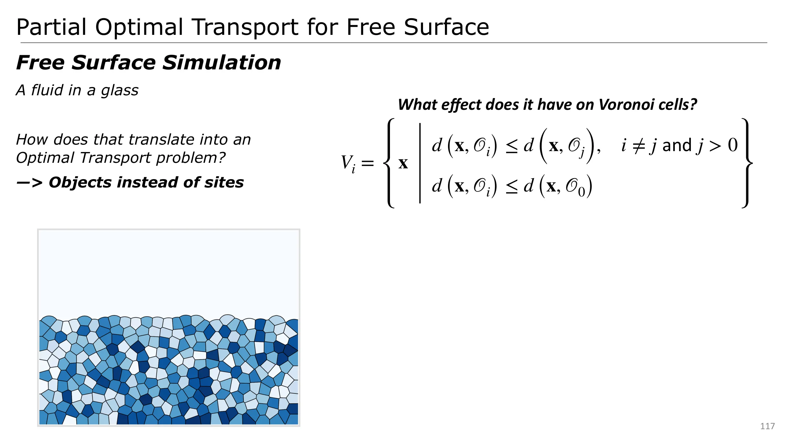
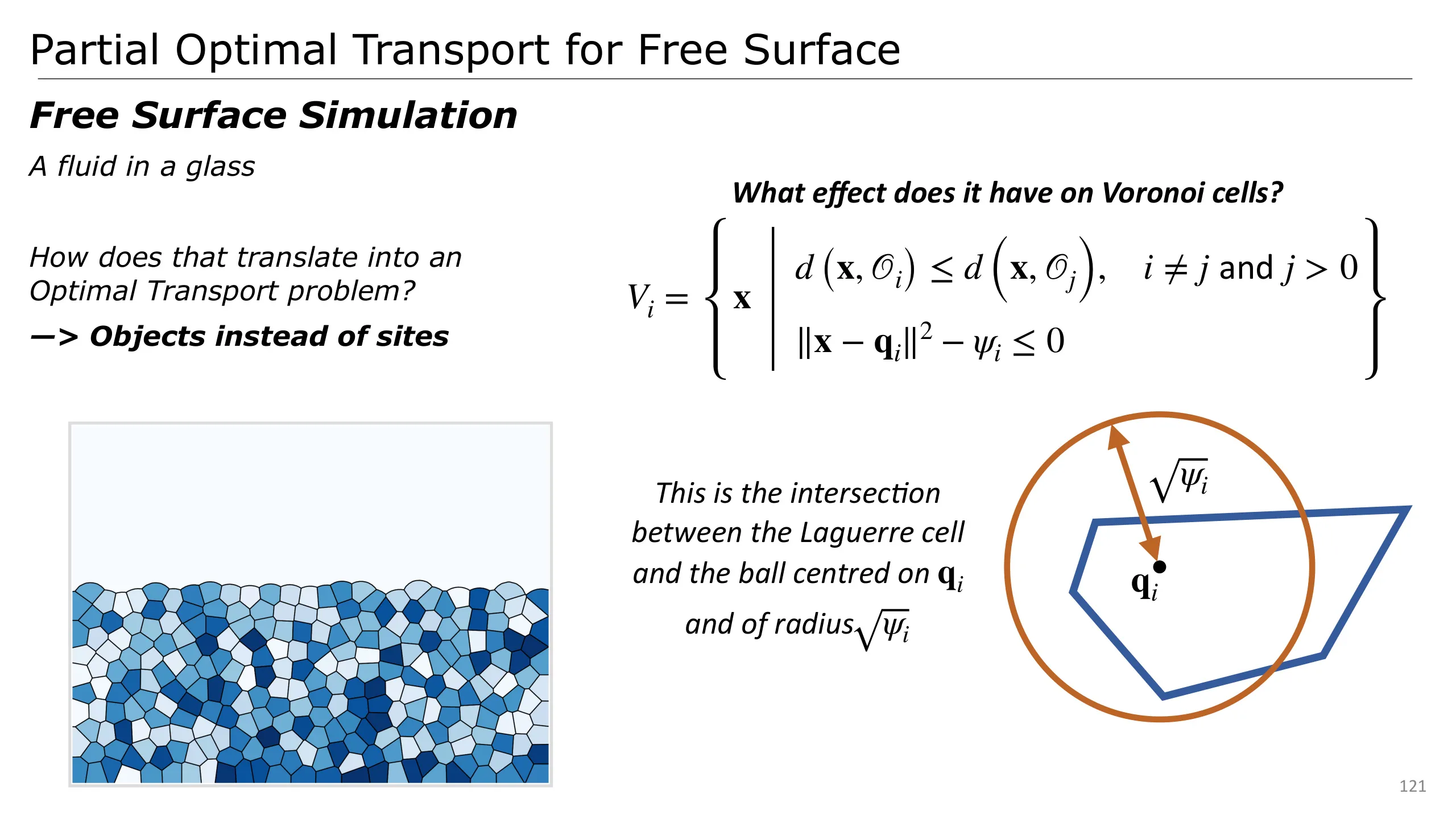
To actually see how it fits an optimal transport problem, we can consider objects instead of sites.

So let’s say that the domain is object 0

And our Laguerre cells the objects of index greater than 0.

The volume linked with the cell 0 is the remaining volume that is not filled with fluid.

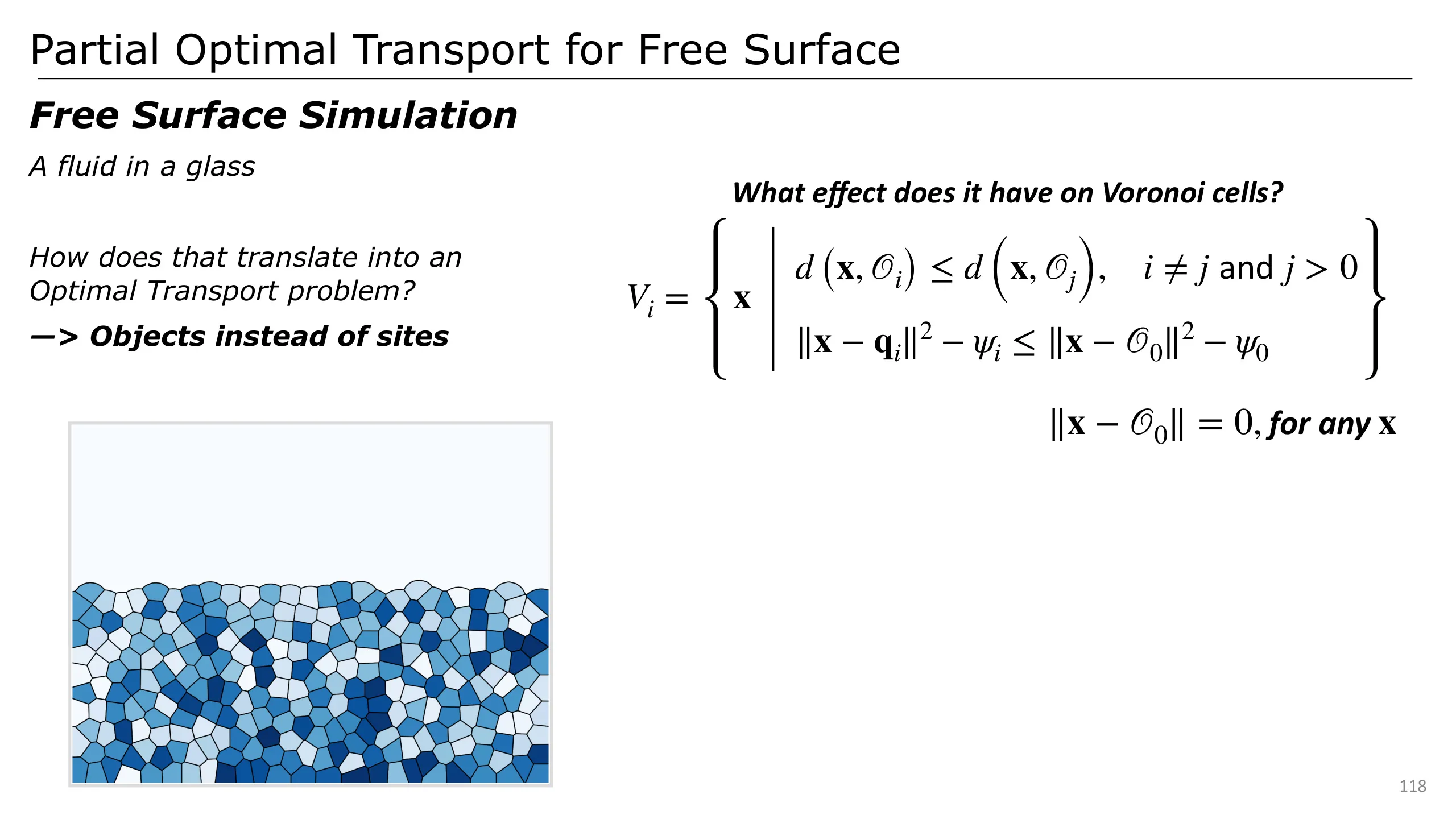
Additionally, since object 0 is a continuum everywhere in the domain, we know that the distance from this object to any point is 0.

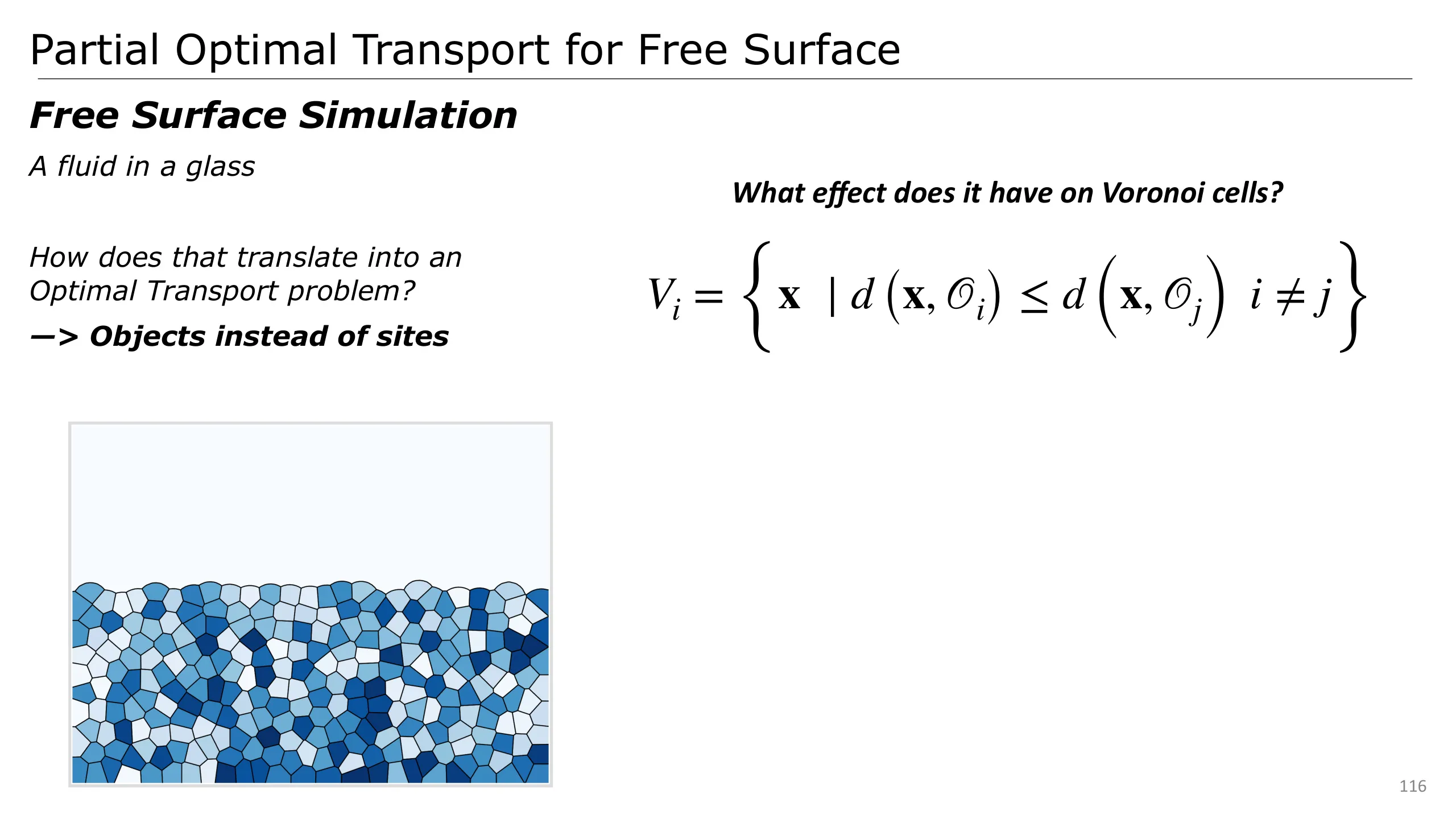
We can now study what happens to our Voronoi cells

Let’s split the constraint to separate the standard sites and the air object on which we have some prior.

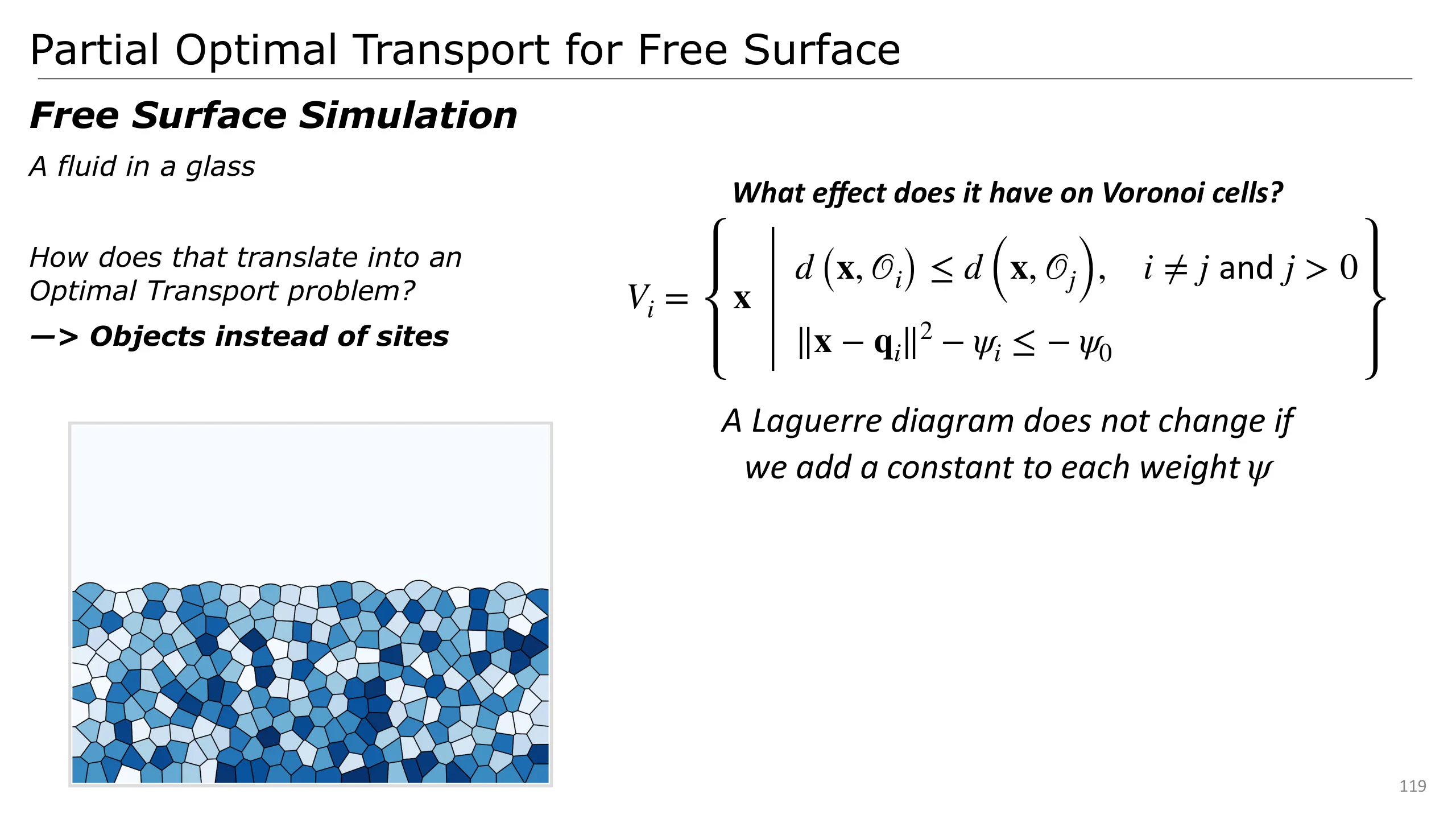
We know that the distance between any point and object 0 is equal to 0, so we can actually remove this term.

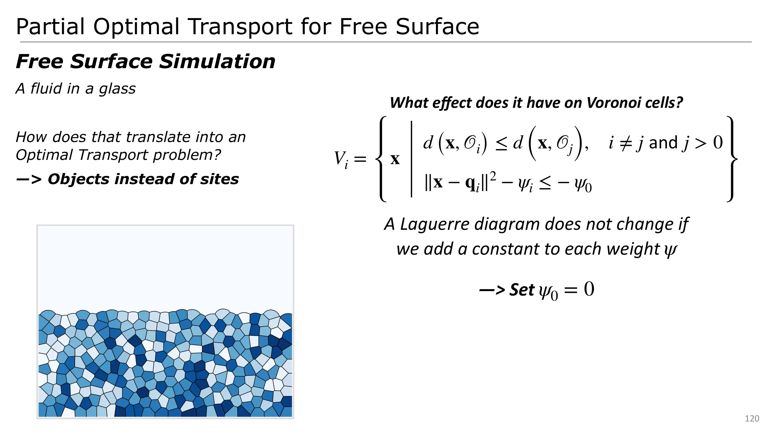
It is a property of Laguerre diagrams that we can add a constant to each weight without actually changing the diagram.

So we can pick psi 0 = 0 without loss of generality!

We obtain another constraint: the Voronoi cells are characterised by the intersection between the original Laguerre cells and the ball centred on qi and of radius sqrt of its weight

To better see why, remember that we said earlier that a power diagram can be lifted to a higher dimensional space as we can see on the right schema by representing the distance functions.

When we look at them from below, we see the image on the left.

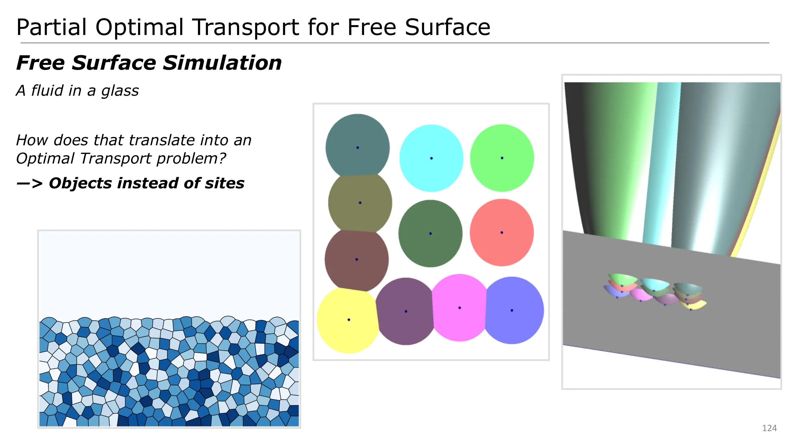
Increasing the weight of a cell yields to a larger cell, which also means that the graph of the distance function is here going down.

Considering our problem with the background object, this results in a clipping of the distance function by our background object which is the plane at z=0

This representation is nice because it gives a very nice idea of what is going on.

This is also nice because we have now an explicit representation of a free surface fluid!

Let’s now see how to compute it.

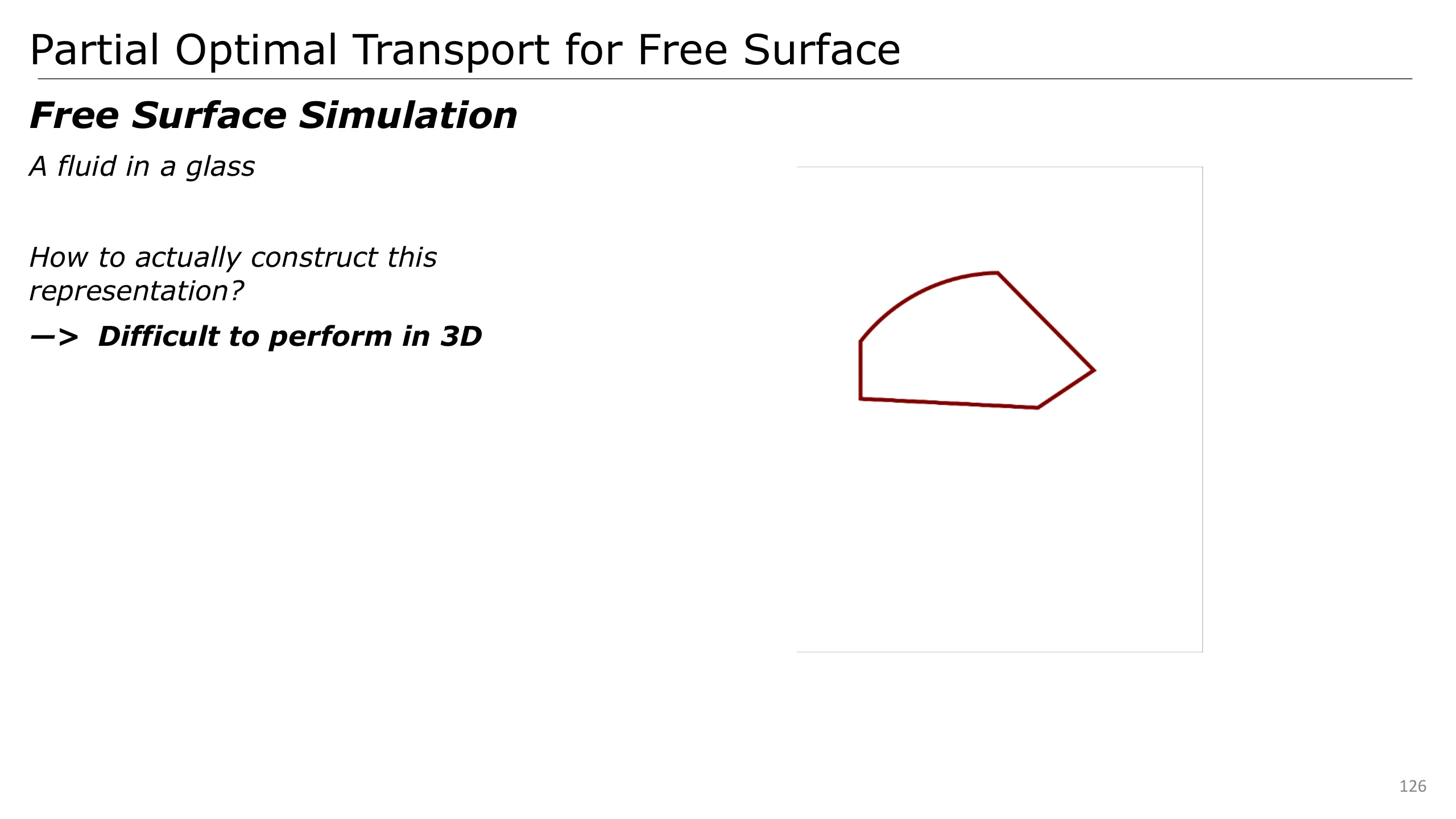
If we consider our problem, we must now clip the cell to obtain the geometry of the Laguerre cells, which must then be clipped by the circle characterised by the site.

The problem is that in 3D it is a complex problem, and we could prefer a simpler method.

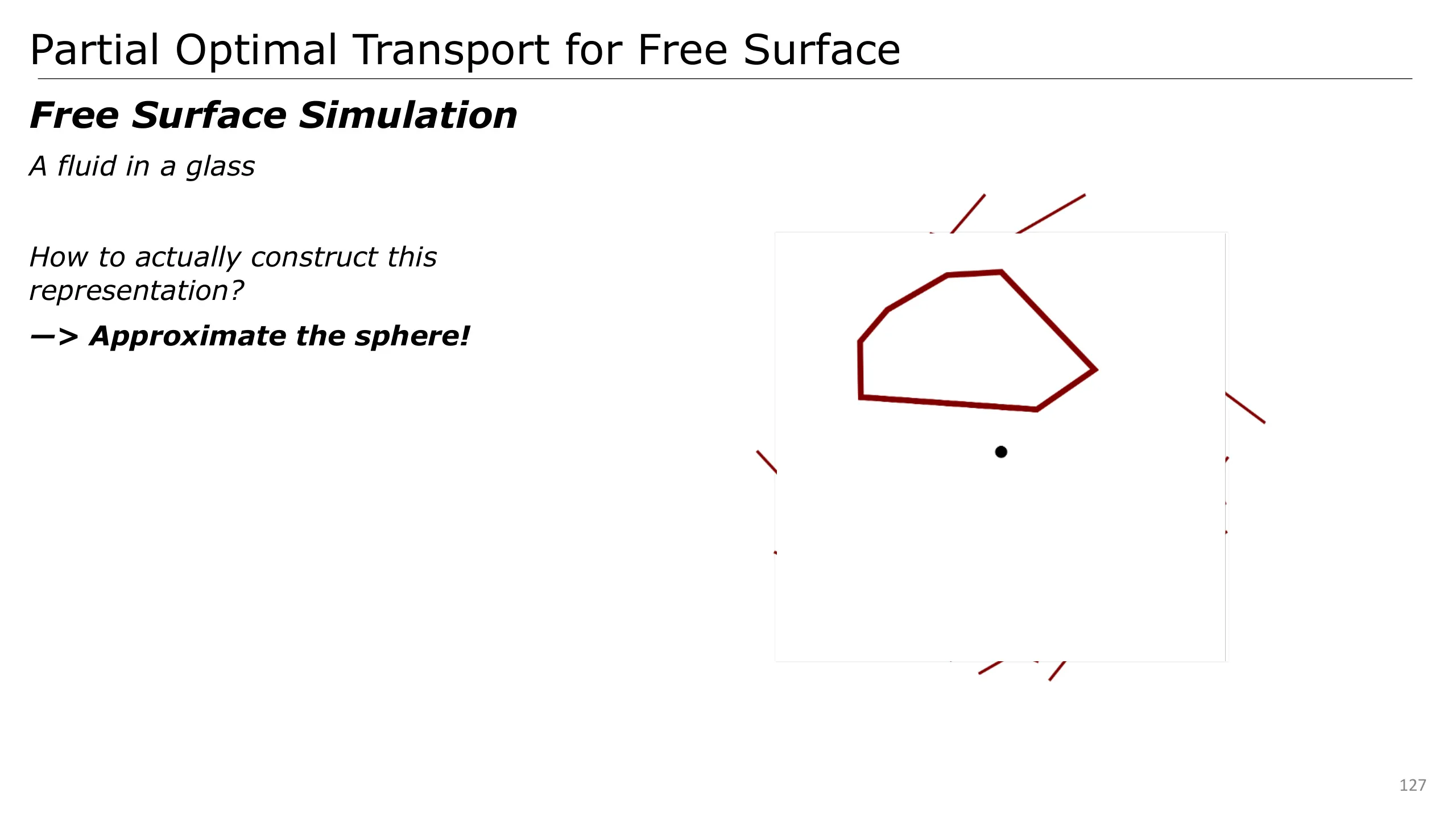
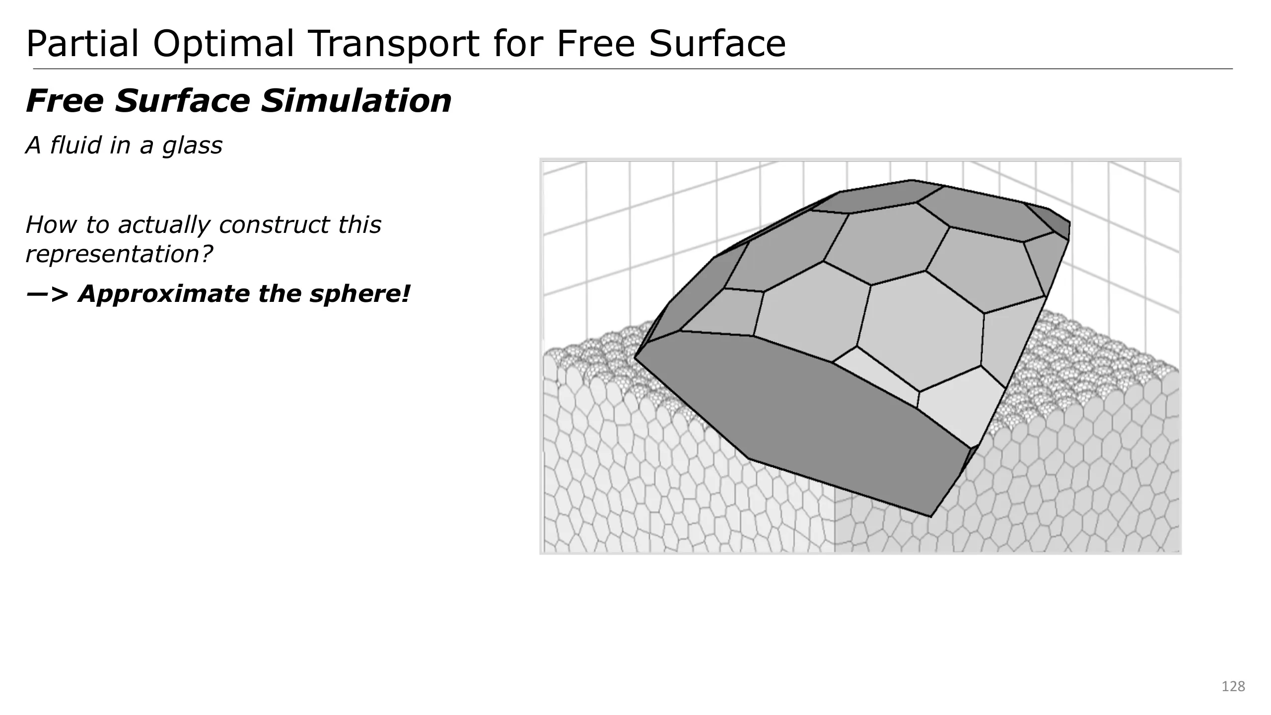
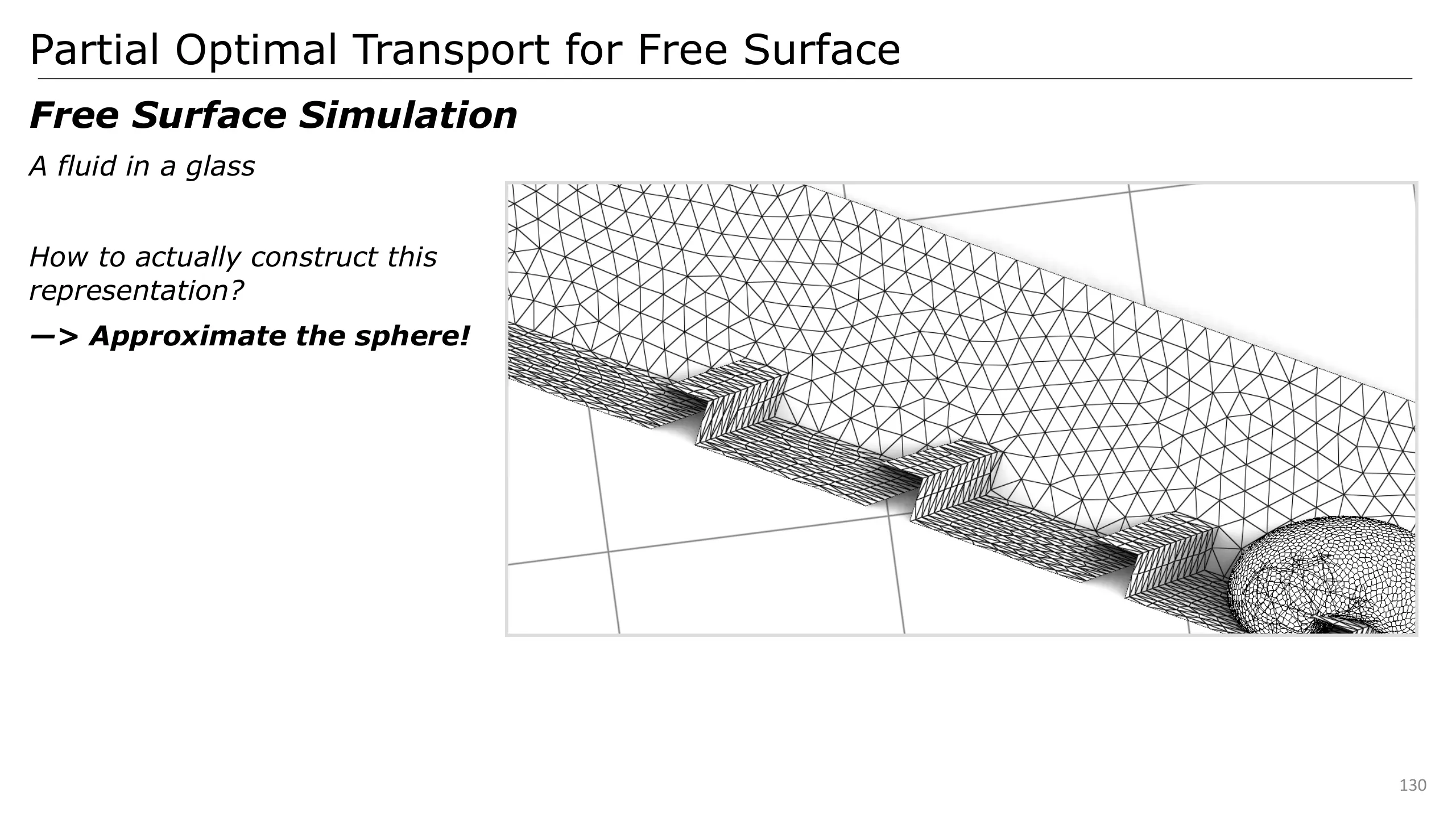
Instead, we can consider an approximation of the sphere with some tangent planes. We can then directly reuse our cell intersection implementation.

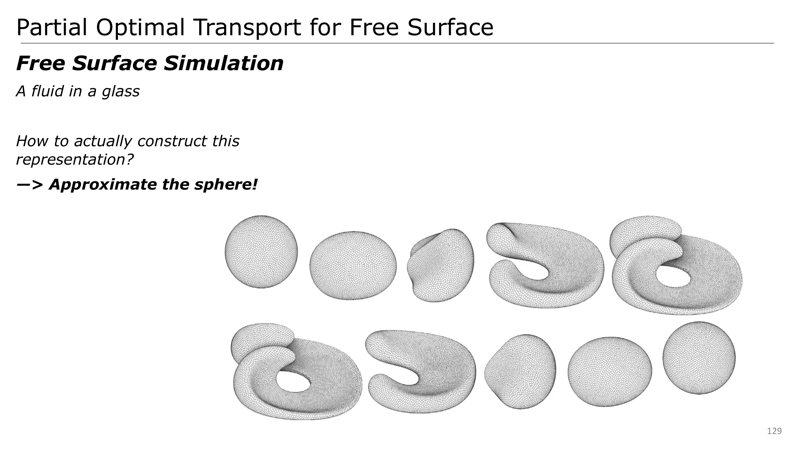
In 3D, it results in such modelling of the fluid, which is composed of Laguerre cells clipped by discretized spheres.

This can represent complex shapes like in this deforming example showing the variety of shape we can represent through this geometry.

And even reproduce this animation reproducing a real experiment!

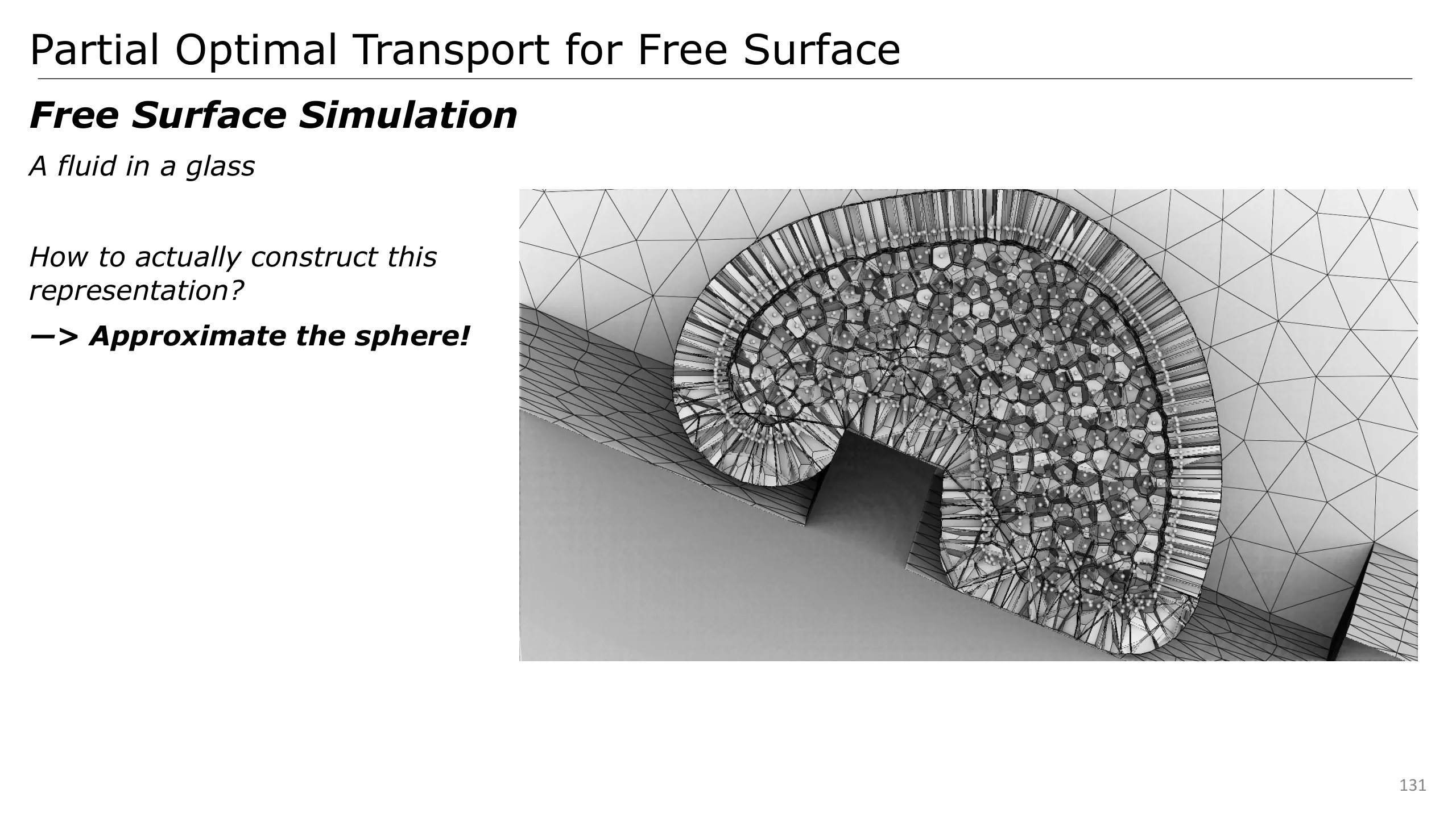
Clipping the geometry, we can see the inside of this droplet.

The boundary cells are clipped by the spheres, which allows modelling this droplet, while the inside cells are just Laguerre cells since they are completely inside their clipping sphere.

Once that we know how to solve a semi-discrete optimal transport problem, one important problem is how to make things work at a larger scale.

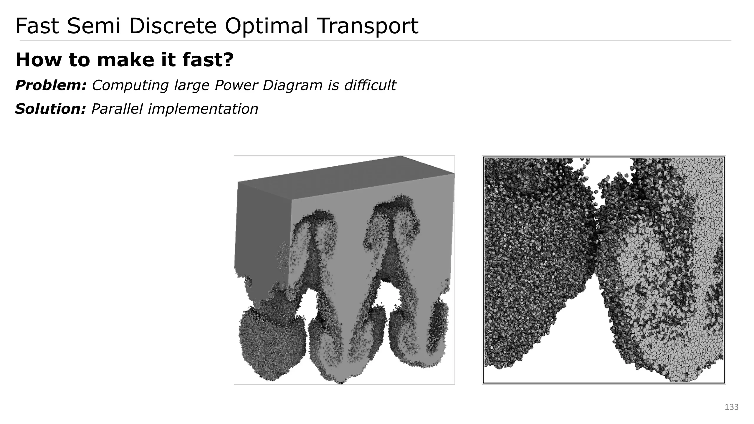
Notably, considering the simulation on the right, we can see that cells become increasingly small and their number increases a lot.

A direct solution is to consider parallelization to benefit from a higher computational throughput.

For that, we can consider two ways: multi core CPU parallelization (or coarse grain) and GPU parallelization.

For that, we must first discuss what we want to compute.

A Power diagram can be represented in two ways:

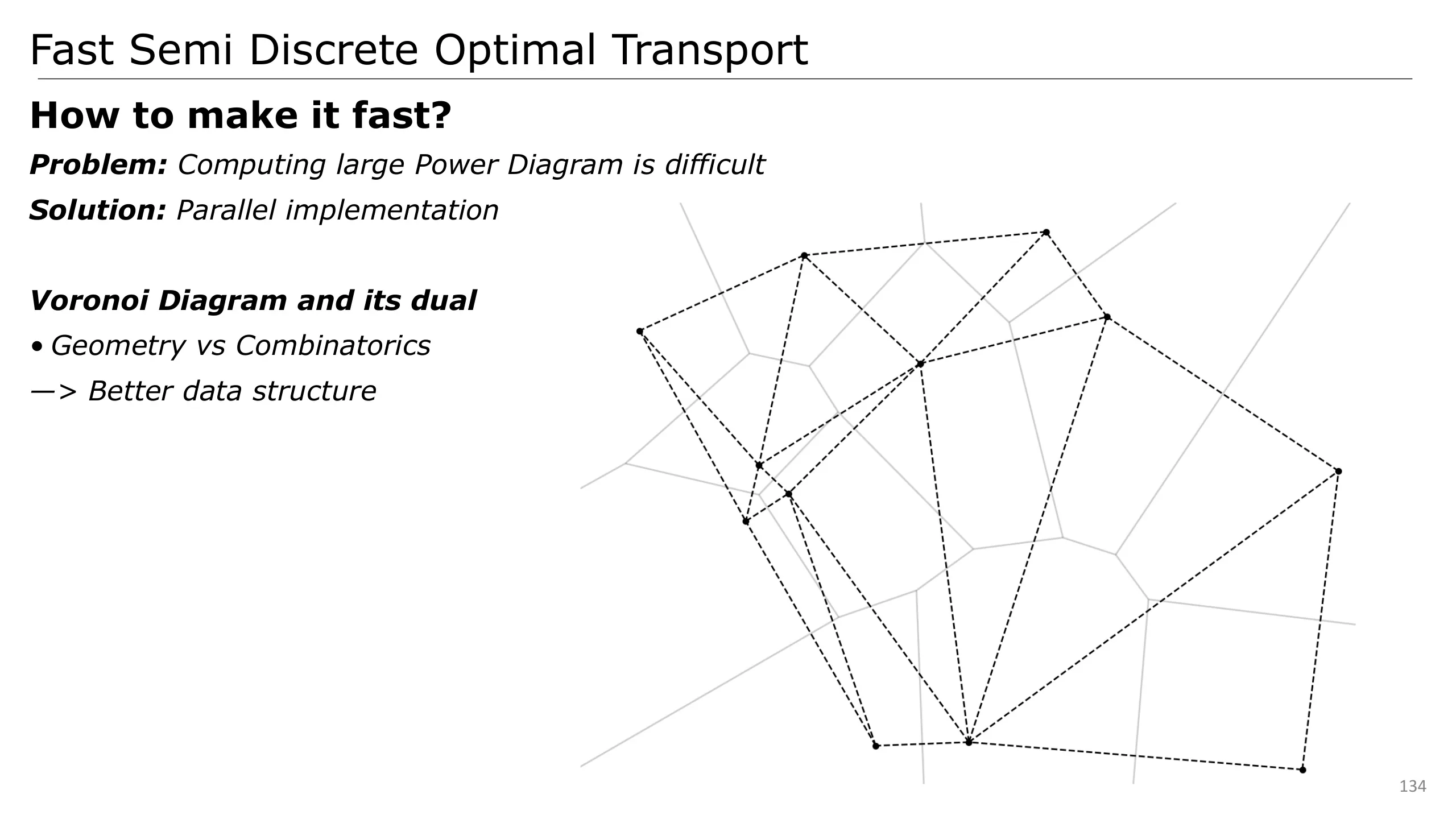
Its geometry, i.e. the set of its cells.

Its combinatorics, or its dual which is a triangulation. When we are talking about a Voronoi diagram, this dual is called the Delaunay triangulation, while considering a Power diagram yields a Regular triangulation

Explicitly storing one or the other has high consequences on the algorithms and the data structure we will be able to manipulate.

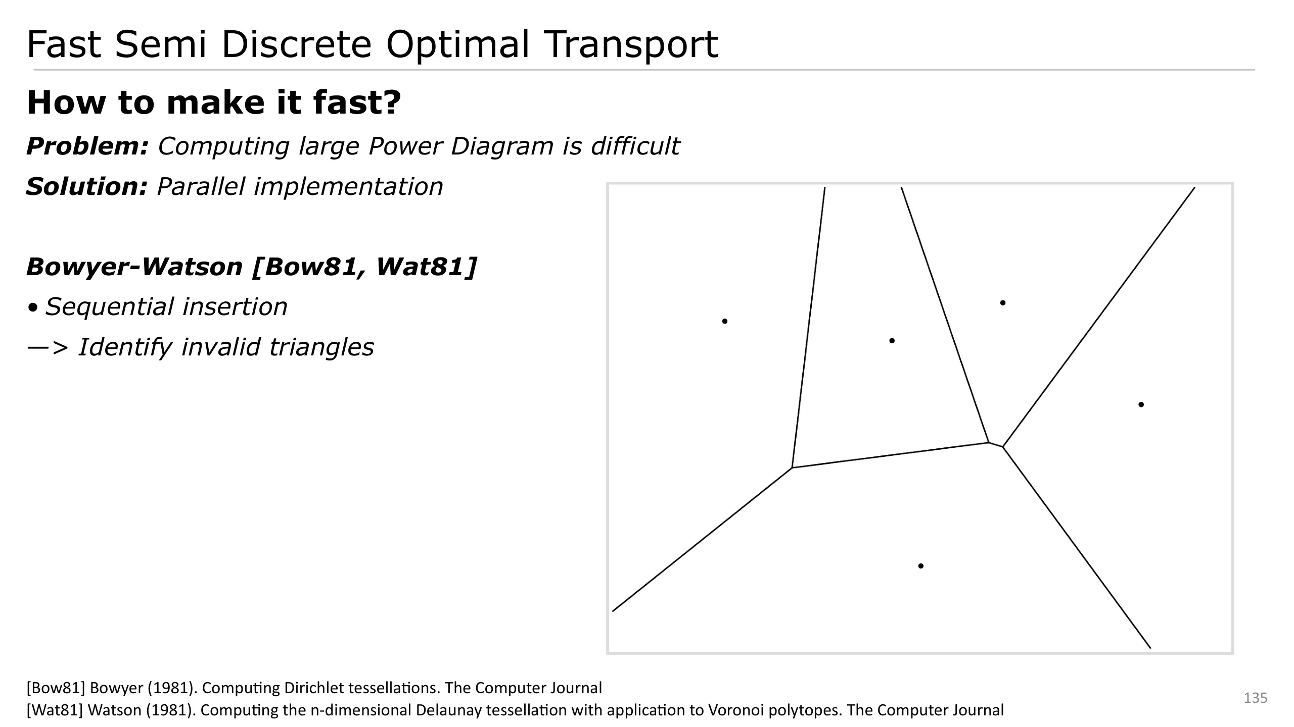
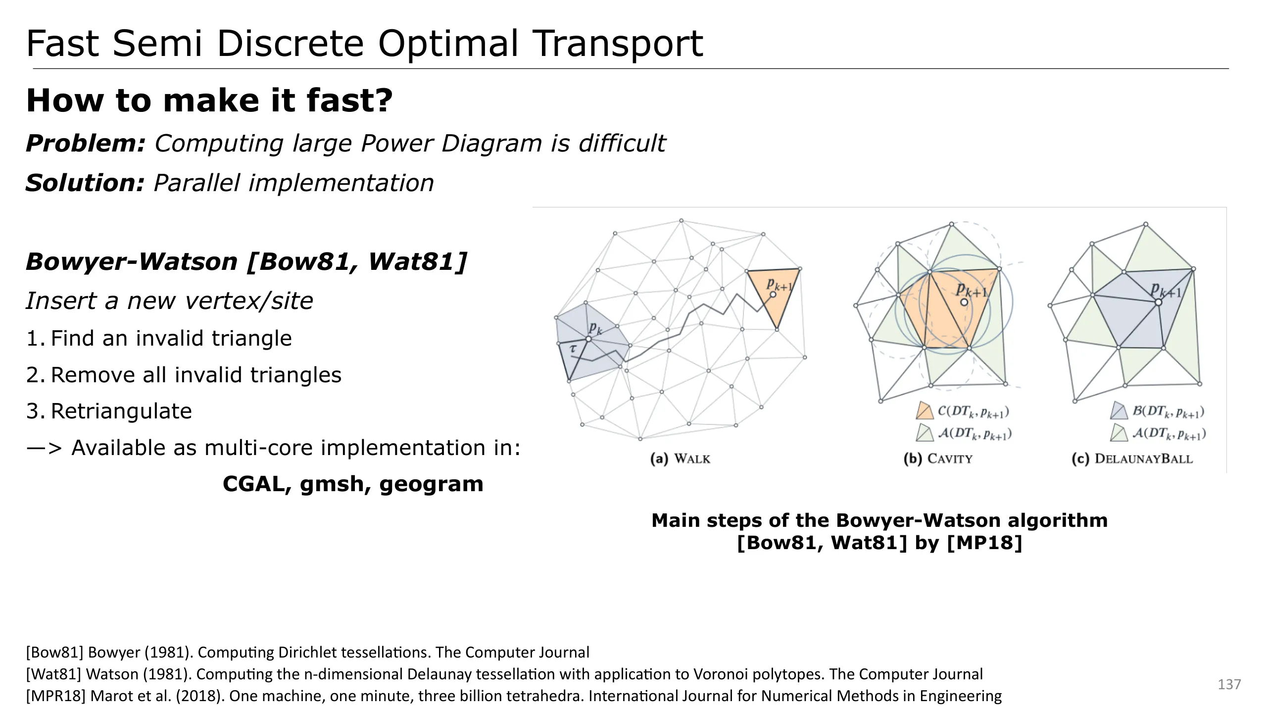
A classic way to compute Delaunay triangulations and Regular Triangulation is the Bowyer Watson algorithm.

This algorithm is based on a sequential insertion of the site to the triangulation.

It then works by inserting one site by one site into the structure by modifying it.

For that, we can consider the characteristics of the Voronoi diagrams.

A vertex of a Voronoi diagram is a point at equal distance of d+1 sites (here 3).

By inserting a new site, we know that existing vertices are invalidated or remain valid iff their closest sites are still their 3 sites.

We can illustrate that by plotting the circle, centred on the vertex and of a radius its distance to its closest sites. If the circle contains the new site, it means that it is closer to the vertex than other sites, and thus, invalidates the vertex.

Here, we observe that the new site in red invalidates one vertex (the red circle).

We can then use that to update the diagram.

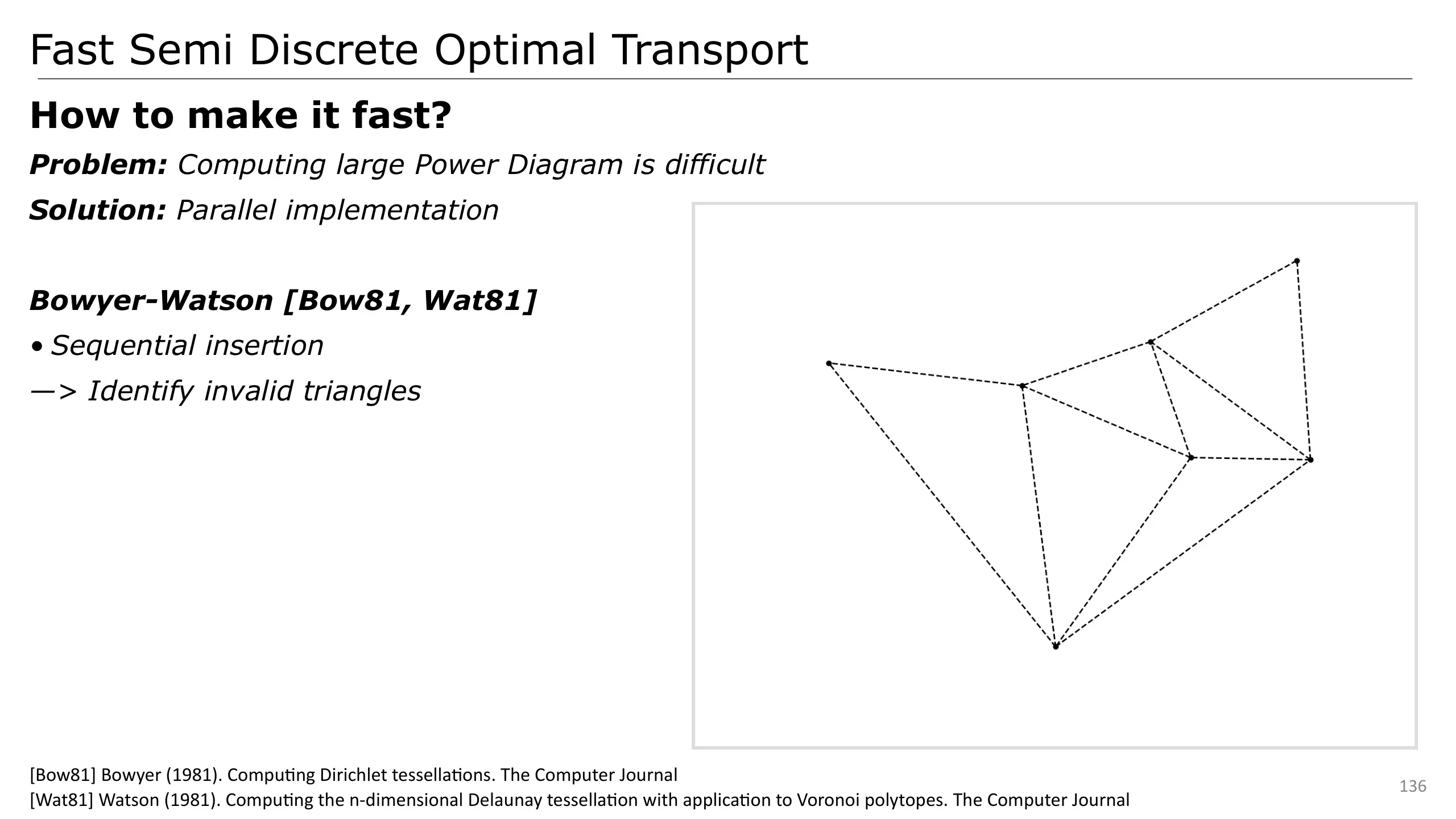
This is especially handy when using the dual of the Voronoi diagram, a Delaunay triangulation.

We can use the rule of the empty sphere (here the empty circle) that is checking if the Voronoi vertex corresponding to a triangle is valid.

We can then remove all invalid triangles

And retriangulate the region with the deleted triangles.

The problem is that this algorithm, naively implemented, must check all vertices/triangles of the diagram.

To make it more efficient, we can use the fact that all invalid triangles are next to each other.

The algorithm then starts by finding a single invalid triangle, and then finds all invalid triangles by checking its neighbors.

It then deletes those and retriangulate the zone.

To further optimize the insertion, it is also possible to sort points spatially, reducing the cost of searching invalid triangles since they are close to each other.

This algorithm is now available in several state of the art libraries as a multi core implementation.

The problem is that it is very hard to implement on the GPU since the data structure is global and it requires a lot of synchronization.

We must then find another point of view.

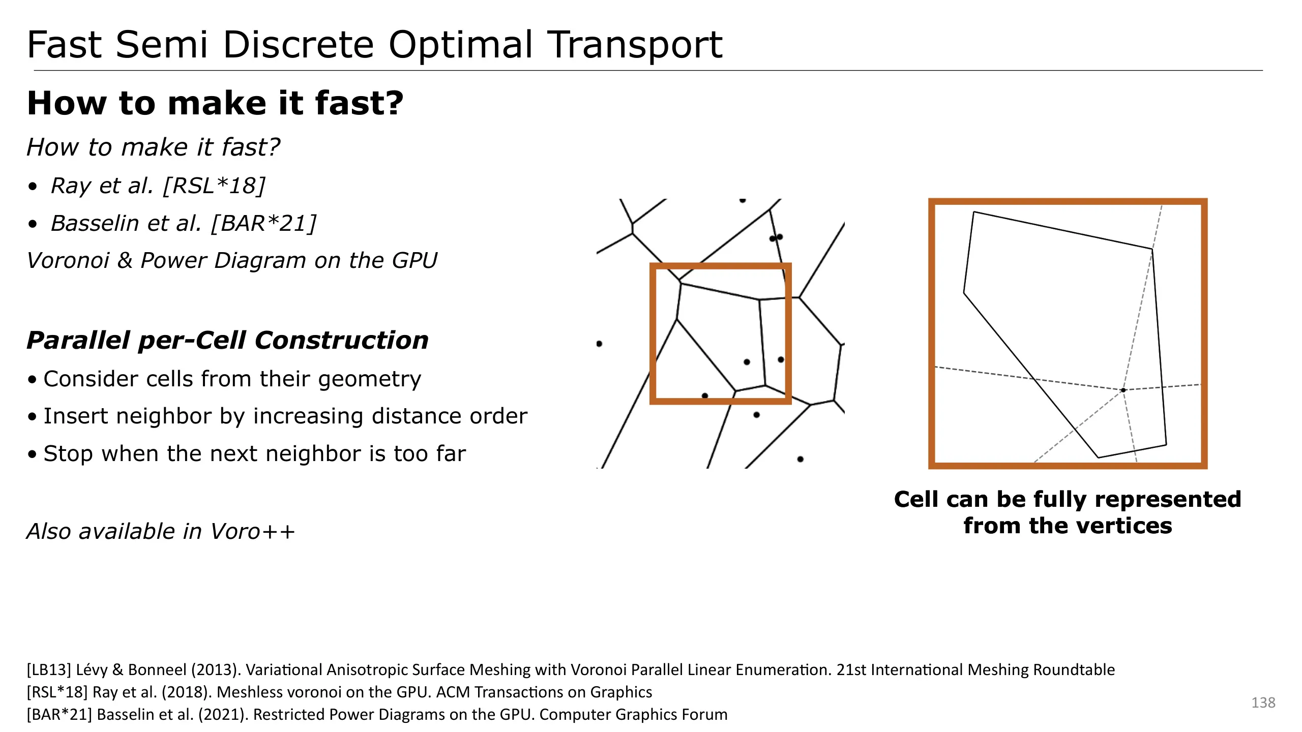
Another line of work, first introduced by Ray et al., considers instead the geometry of the diagram : i.e. its cells.

Those can be fully represented and stored from their vertices which is very compact.

By storing them individually, this enables a cell-wise parallel implementation which suits very much the GPU.

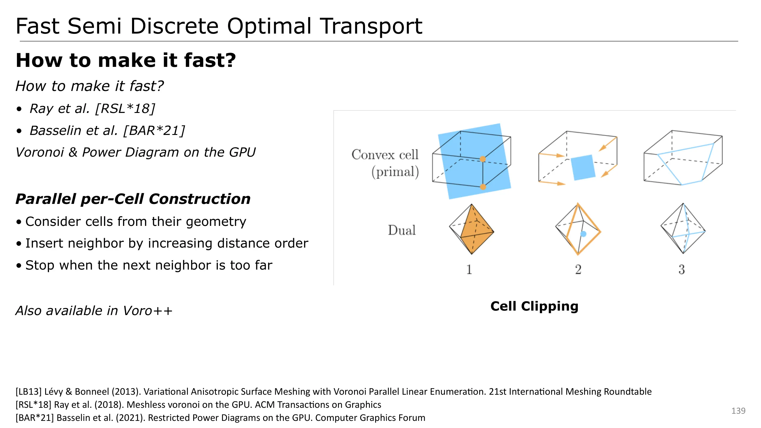
A neighboring site can be inserted to a cell by clipping the cell with the bisector between both sites, which can be made efficiently based on the list of the cell’s vertices.

We can then initialize the cell with a very large bounding box, usually the domain, and insert its neighbors by increasing distance order.

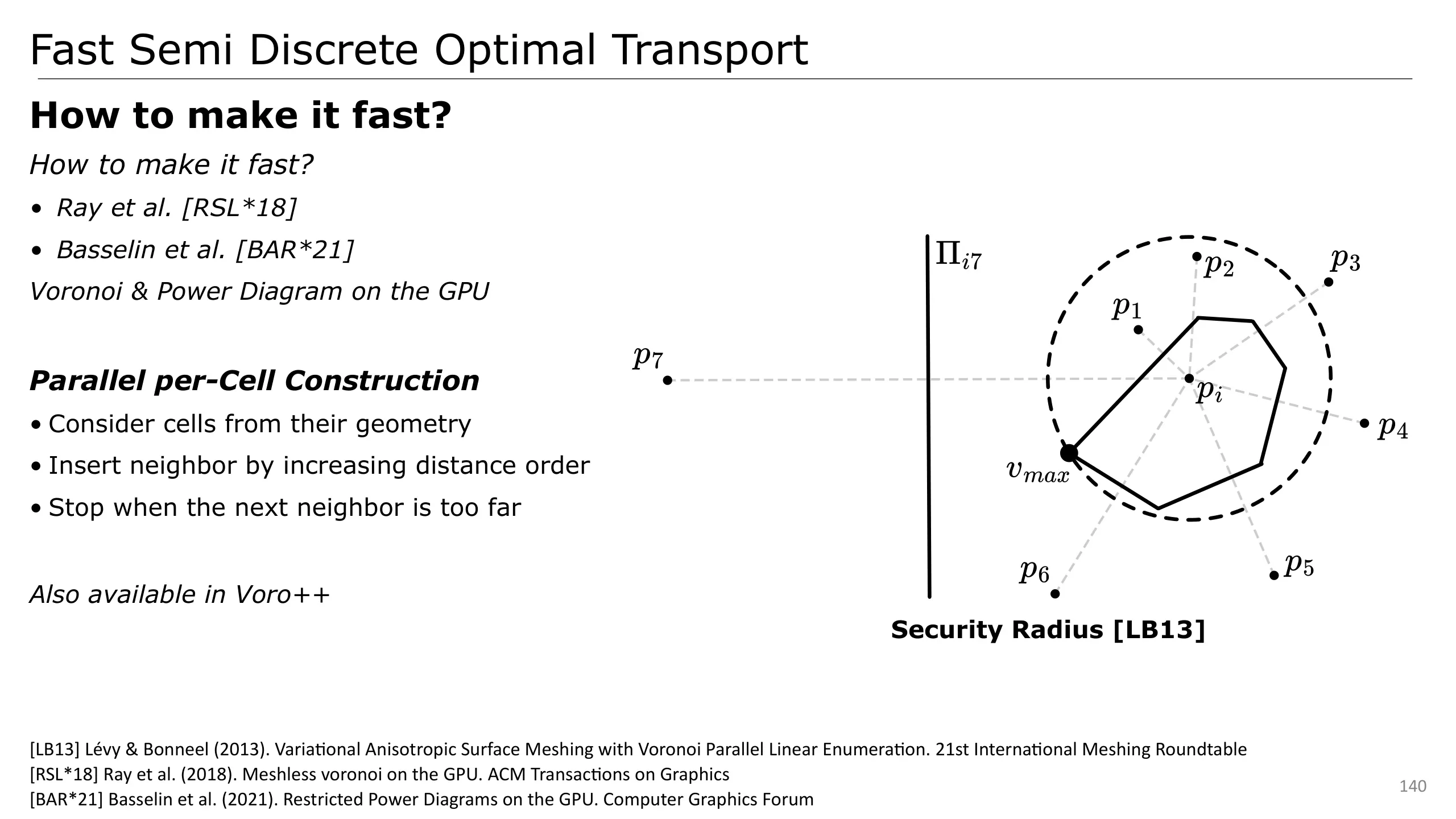
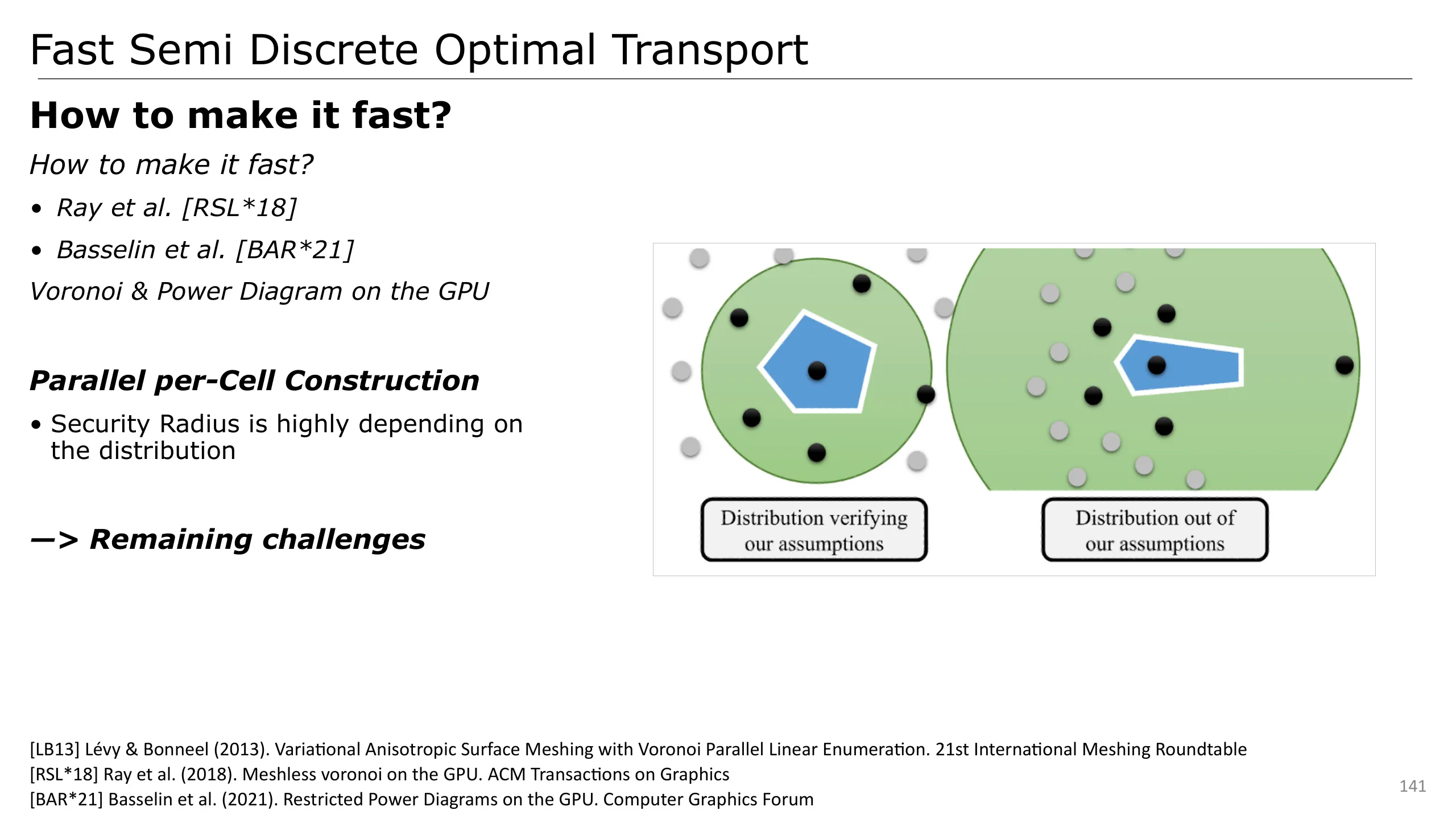
The insertion can then be stopped based on a criterion named the security radius. This criterion states that if the next neighbor distance is sufficiently far away, it will not contribute and thus, we can stop the search.

This method yields very nice results but there is one problem, it is highly linked on the assumption that the distribution of site is very homogeneous.

As we can see on this schema, when the neighbors of a cell are located in a spatially heterogeneous way, it will yield a large security radius which will make us consider a lot of neighbors that will not contribute to the cell.

This impact has been studied by Ray et al., which provides many interesting remaining challenges.

Working with the cell of the diagram has other nice advantages.

Notably, to solve the Optimal Transport problem, we must perform an integration per-cell.

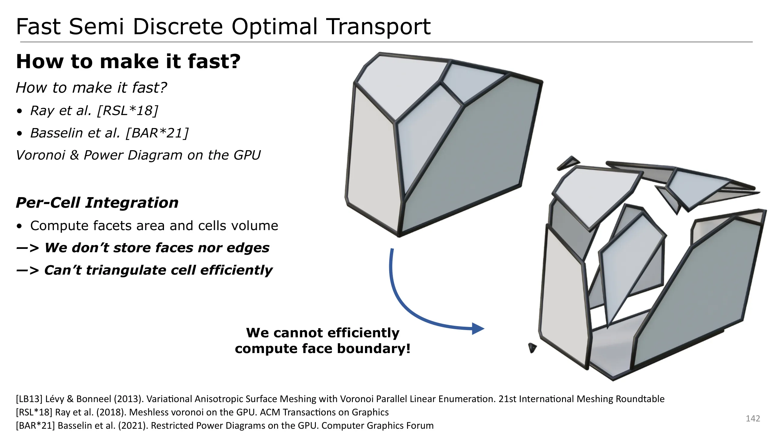
The problem is that, to do that, we must compute the volume of the cell and the area of the facets.

This is very easy when we don’t really care about the data structure, but here we want to be as fast as possible. We can’t really afford to change our data structure.

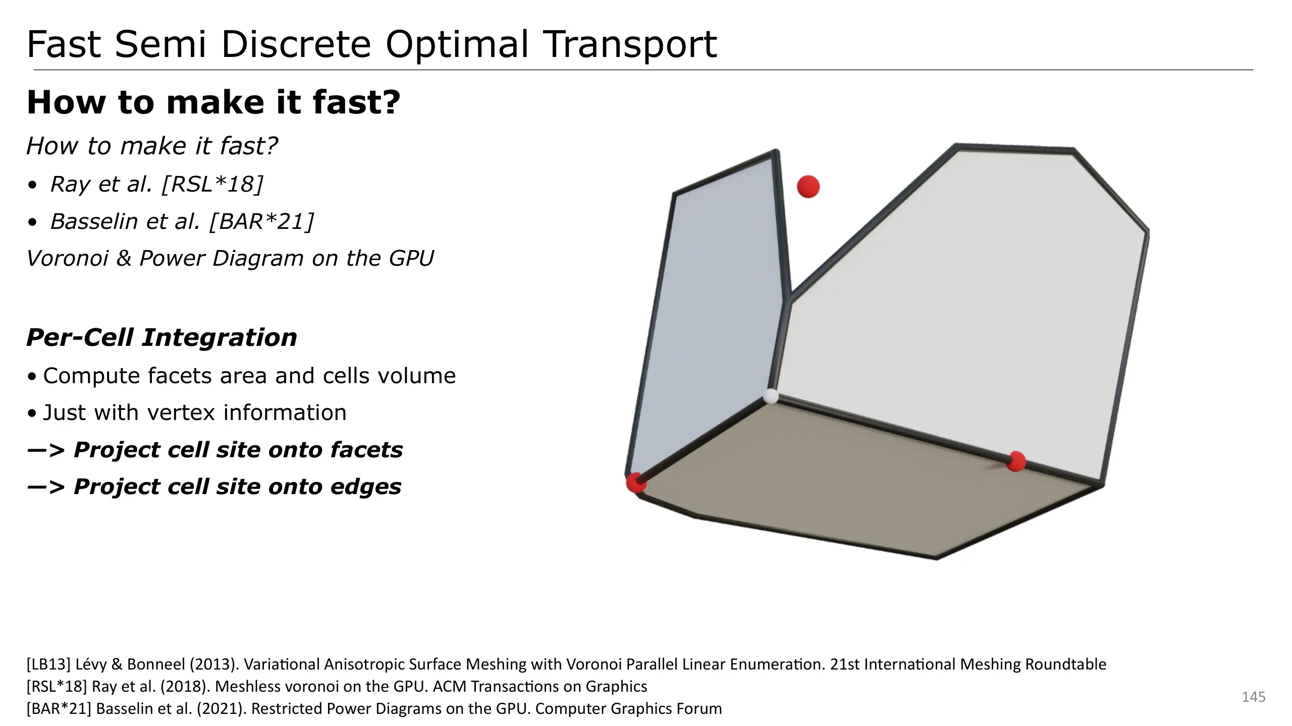
The problem then is that we only store vertices, and we don’t have information on faces nor edges. We also can’t triangulate the cell efficiently.

Ray et al. proposed an alternative POV which has very nice properties.

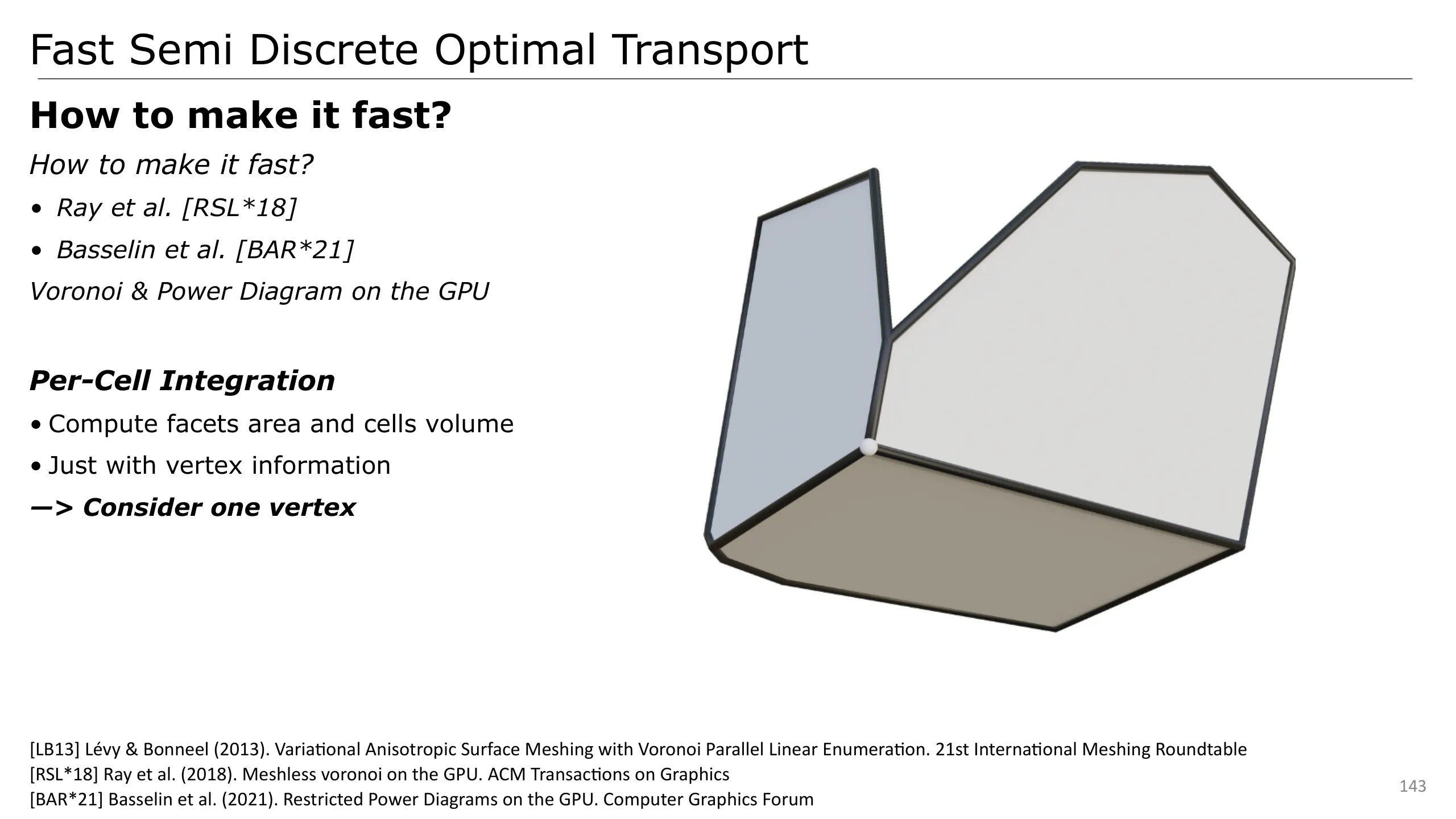
First, let’s say we want to compute the cell volume and facets area independently, just by considering the vertices of the cell.

Let’s consider a first vertex.

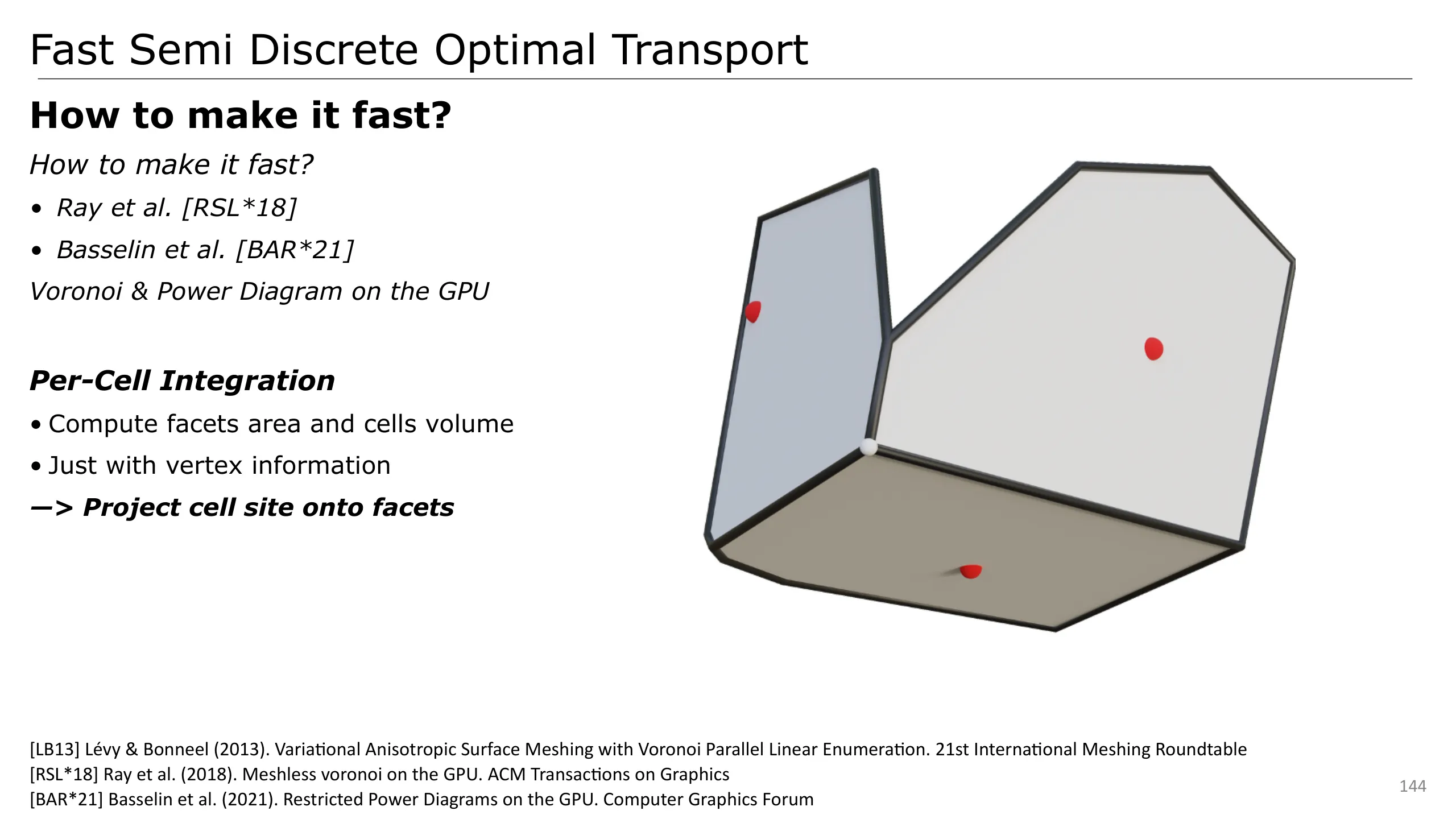
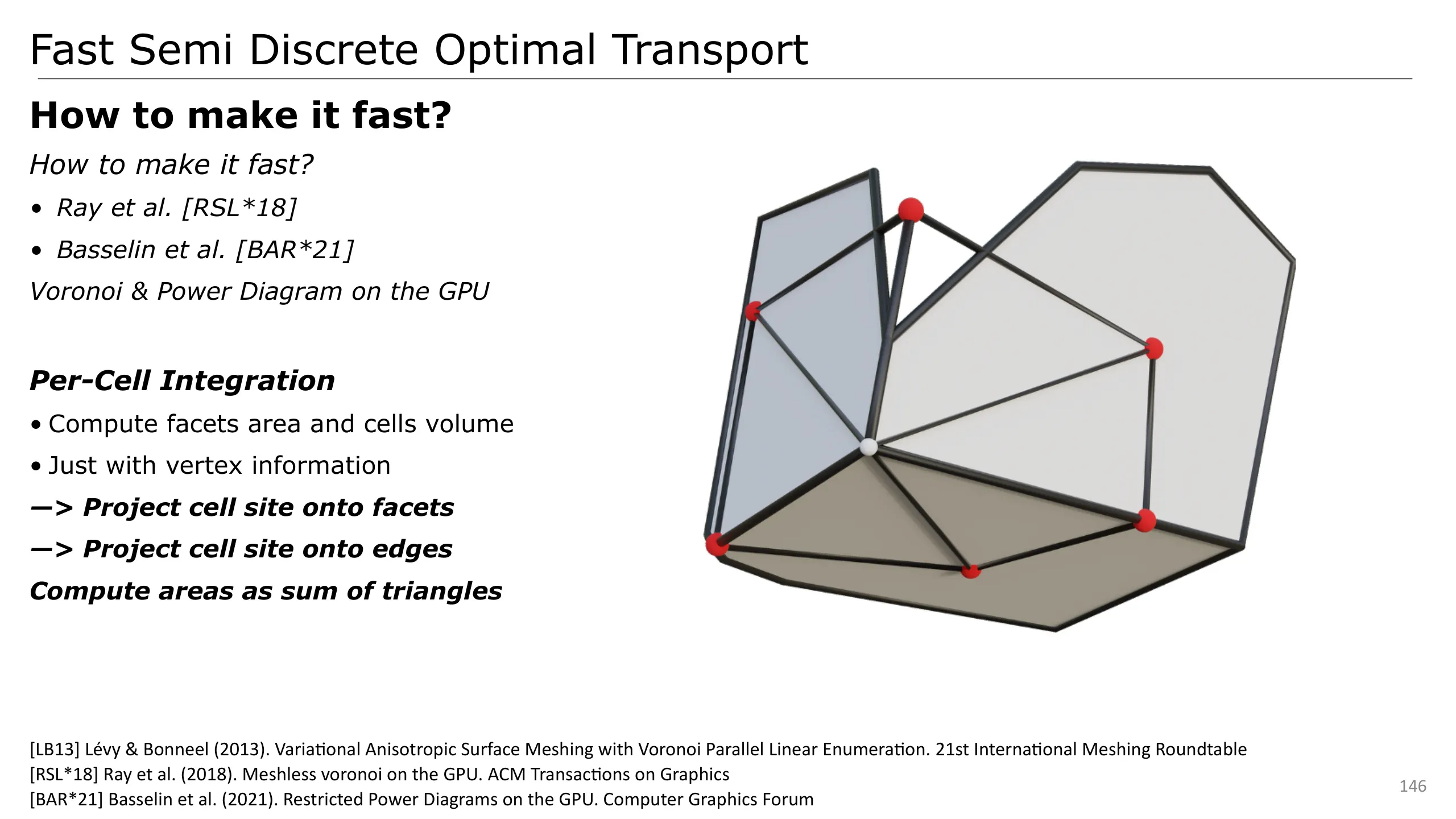
We can project the current site of the cell onto the related facets of the vertex (in red).

And also on the edges related to our vertex

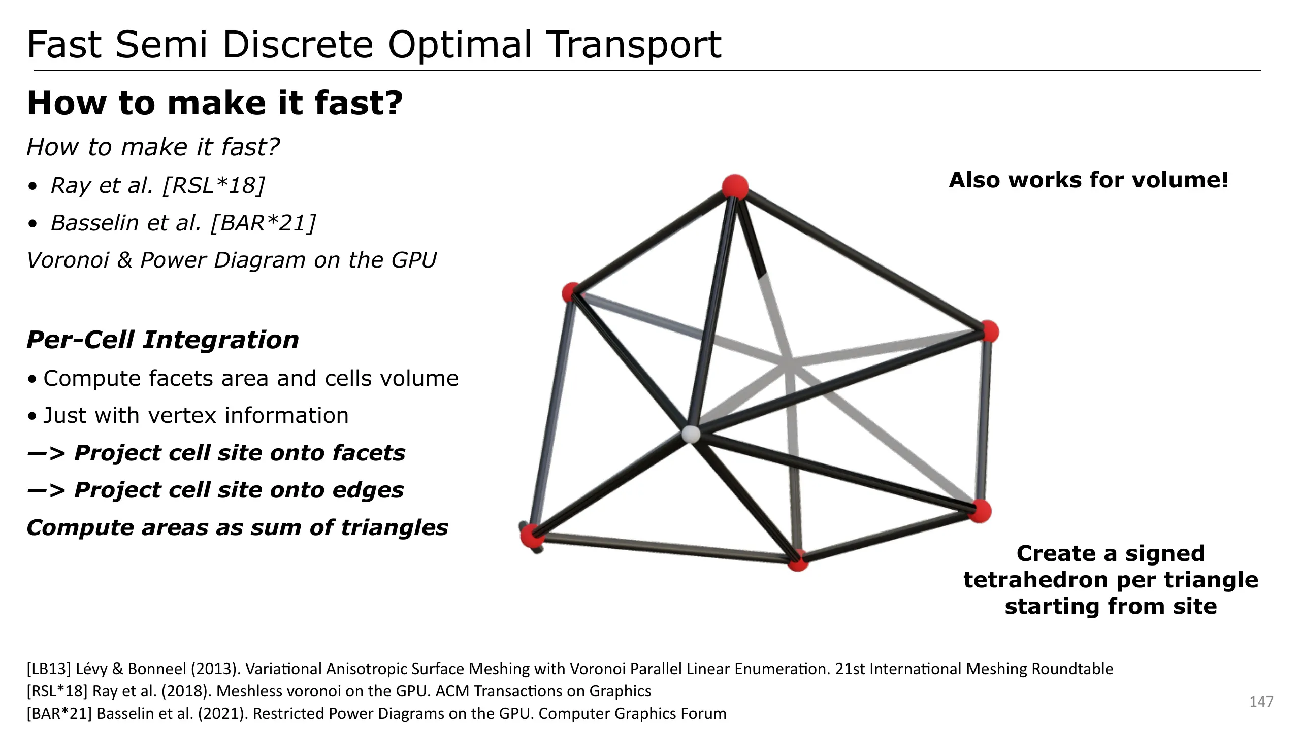
Notice that this decomposition is only valid by considering signed area as we can see on this figure.

Parts of some triangles are going out of the cells, but as others will be negative, their sum will be equal to the area we want to compute.

What is very cool is that it also works for the volume of the cell by considering a tetrahedron per triangle starting from the site.

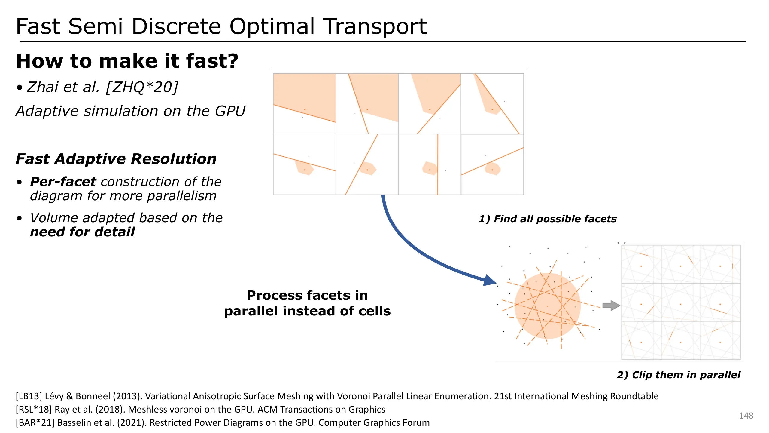
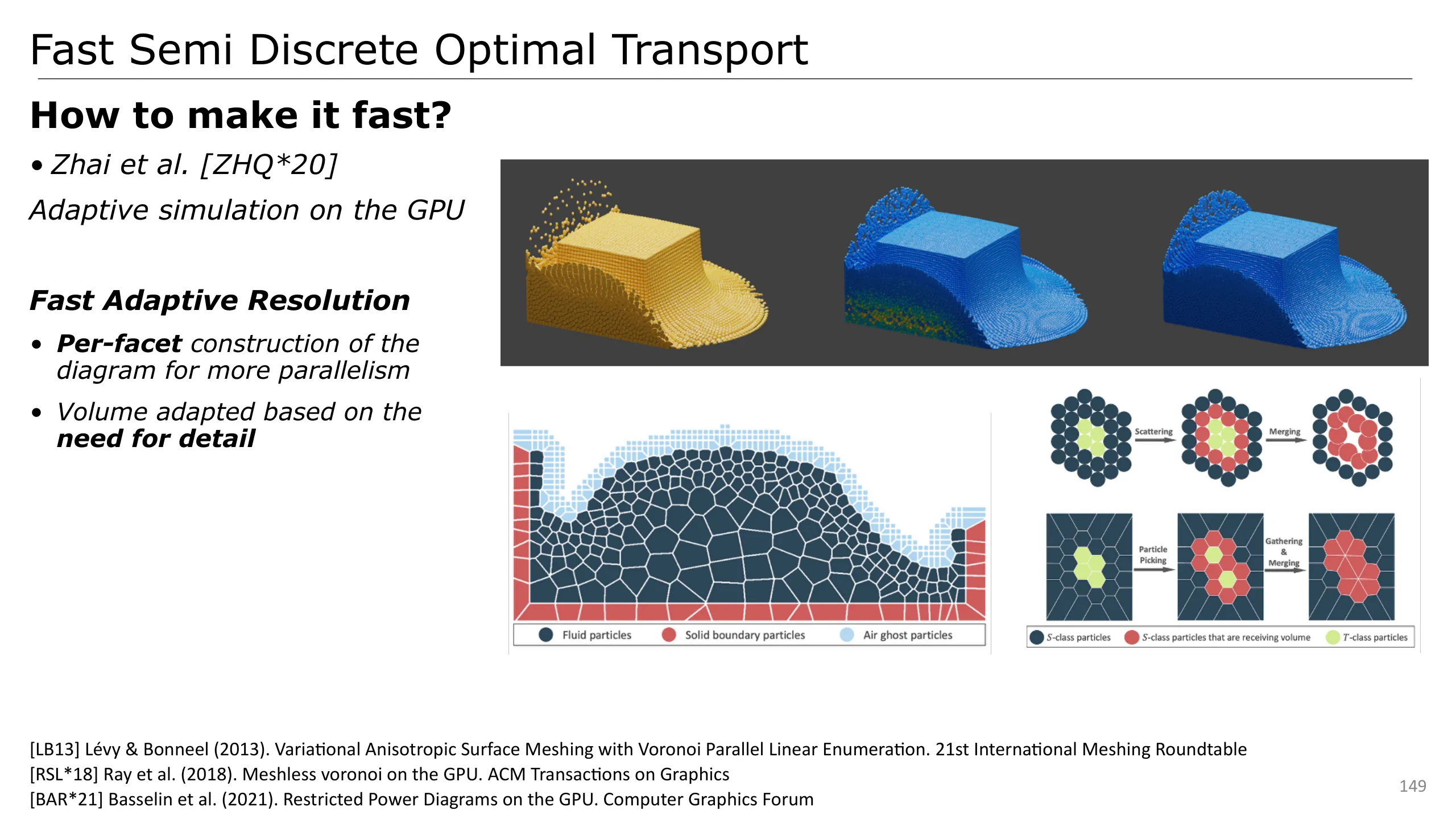
In this context, Zhai et al. added further improvements

First, considering only cell can be quite inefficient in terms of parallelism on the GPU. Indeed, some cells may require more work than others which may lead to imbalanced dispatch.

To address these issues, they first compute all possible facets of the cell, and process them in parallel. This yields a simpler work per cell and improves the parallelism.

Additionally, they propose to adaptively sample the matter where details are required.

Since we have a very precise way to control the volume of each cell, we can assign a larger volume of matter where we don’t need detail, and the other way around.

This results to detailed simulation at a reduced cost.

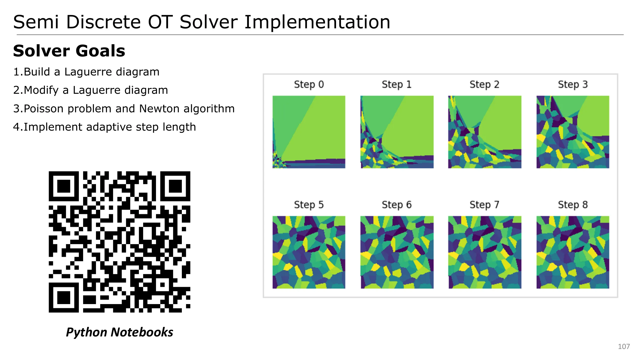
This ends this tutorial. If you want to dig a bit more into this, we provide an implementation of Gallouët and Mérigot’s scheme at the following address.